where hi and hj are two data points and φ· is the feature mapping function. To make data set H away from the origin, equivalent to the following optimization problem Equation 8:

minw,ξ,v12||w||2+1CN∑iξi−vsubjecttowi:i=1,2,⋯,N , for any of the test sample hp , its corresponding decision function is Equation 9 below: fhp=sgn∑iwikhphi−v    (9)

Where sgn· represents a symbolic function. If the decision function fhp=−1 of sample hp is tested, then sample hp is diagnosed as normal. Conversely, if the decision function of test sample hp , then test sample hp is diagnosed as an abnormal sample. Thus anomaly detection under unbalanced conditions can be realized.

3.5 Evaluation metrics of the WCOS model

The Area Under the Curve (AUC) of Receiver Operating Characteristics (ROC) was used as the evaluation index, ROC abscissa is the false positive rate (FPR), the ordinate is the true positive rate (TPR), and the area surrounded by the coordinate axis is defined as AUC. Studies show that AUC can better measure the performance of the classifier than the overall accuracy under the condition of uneven data. AUC is an index to evaluate the quality of the binary classification model, given by Equation 10:

AUC=∑i∈positionClassranki−M1+M2M×N∑i∈positionClassranki    (10)

where positionClass represents the positive set, ranki represents the rank of the ith sample in the sample ranking, and the ∑i∈positionClassranki term represents the sum of the ranks belonging to the positive samples. M and N represent True Positive Rate (TPR) and False Positive Rate (FPR), respectively.

4 Experimental results 4.1 Data set preparation and preprocessing

To verify the validity of the constructed heart sound abnormality detection model, a Littmann 3200 electronic stethoscope from 3 M Company, USA, was used to collect heart sound signals to construct the dataset. The data were processed using a 5-fold cross-validation method, and the data were derived from actual clinical measurements in multiple medical institutions, not from simulations. In clinical practice, abnormalities in cardiac structure or function are associated with changes in the rhythm, frequency, and intensity of heart sounds. For example, murmurs caused by valvular lesions and weakened or enhanced heart sounds due to myocardial lesions are selected as key indicators for the detection of abnormalities. At the same time, we searched patients’ medical records, diagnostic reports, and treatment feedback to accurately determine the status of heart sounds, constructed samples using sliding window technology, and analyzed a large number of cases to clarify that the length of abnormal heart sound sequences was mostly in the range of 6 to 10, and then set the sliding window size to 10.

This paper is experimentally verified on a device with a six-core Intel(R) Core (TM)i7-9750HCPU@2.59GHz processor and 8GB DDR4 memory.

4.2 Experimental setup

The original signal statistics method TF24 calculates the original signal through a series of specific formulas, and its role is to decomposition the original sound signal into 24 parameters, which cover a variety of characteristics of the signal in the time domain and frequency domain. The main purpose of TF24 is to extract representative features from the original signal, which can describe the characteristics of the original signal more comprehensively. The usage of TF24 is to use its 24 extracted parameters as features as the input of subsequent models (such as OCSVM). The time domain parameters are expressed as p1 ~ p11 and given by Equation 11:

p1=∑n=1NxnNp2=∑n=1Nxn−p12N−1p3=∑n=1NxnN2p4=∑n=1Nxn2Np5=maxxnp6=∑n=1Nxn−p13N−1p23p7=∑n=1Nxn−p14N−1p24p8=p5p4p9=p5p3p10=p41N∑n=1Nxnp11=p51N∑n=1Nxn    (11)

In Equation 11, p1 represents the average amplitude of the signal in the time domain, p2 calculates the standard deviation of the signal in the time domain, p3 is related to some weighted summation of the signal amplitude, p4 represents the root mean square value of the signal in the time domain, p5 directly obtains the maximum amplitude of the signal in the time domain, p6–p11 These parameters involve higher order statistics of the signal amplitude relative to the mean.

In addition, the original signal statistical method decomposed the sound signal into 13 parameters in the time domain, expressed as p12 ~ p24, which is given by Equation 12:

p12=∑k=1KskKp13=∑k=1Ksk−p122Kp14=∑k=1Ksk−p123Kp133p15=∑k=1Ksk−p124Kp132p16=∑k=1Kfksk∑k=1Kskp17=∑k=1Kfk−p163skKp18=∑k=1Kfk2sk∑k=1Kskp19=∑k=1Kfk4sk∑k=1Kfk2skp20=∑k=1Kfk2sk∑k=1Kfk4sk∑k=1Kskp21=p17p16p22=∑k=1Kfk−p163skKp172p23=∑k=1Kfk−p16skKp174p24=∑k=1Kfk−p164skKp17    (12)

In Equation 12, p12 represents the vibration energy in the frequency domain, and p13-p15, p17, and p21-p24 represent the convergence of the power spectrum. p16, p18, p19 and p20 represents the pattern of change of the main frequency.

The experiments involved four modules, namely OCSVM model, raw signal statistics TF24, convolutional autoencoder, and wavelet decomposition. Five models were set up for comparison, the control group is shown in Table 1.

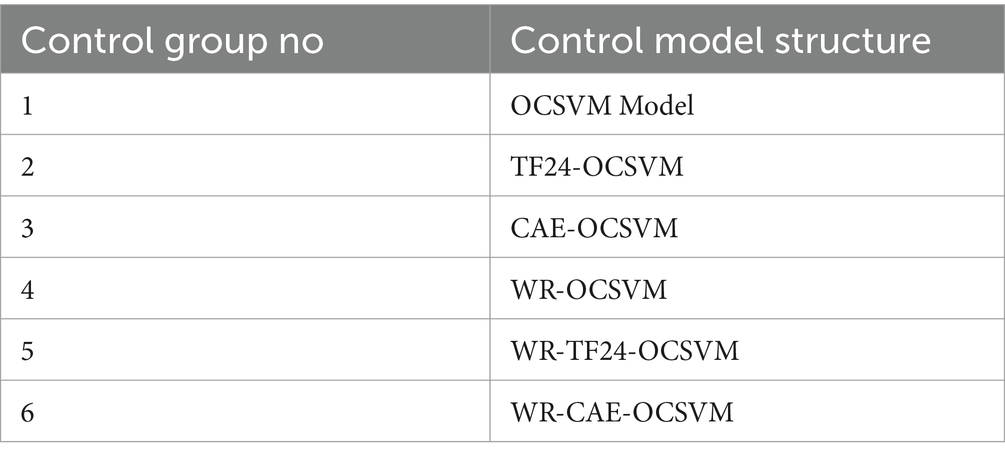
Table 1. Control group setup.

As can be seen in the above table, the first group OCSVM represents a classification support vector machine, the second group TF24-OCSVM represents the combination of raw signal statistical method (TF24) and OCSVM, and the third group CAE-OCSVM represents the combination of convolutional autoencoder (CAE) and OCSVM. The fourth group of WR-OCSVM represents the combination of wavelet reconstruction (WR) and OCSVM, the fifth group of WR-TF24-OCSVM integrates wavelet reconstruction, raw signal statistical methods and OCSVM, and the sixth group of WR-CAE-OCSVM combines wavelet reconstruction, convolutional autoencoder and OCSVM.

4.3 Result analysis 4.3.1 Comparison with other models

Comparing multiple current anomaly detection models, We chose the variant autoencoder (VAE)-based anomaly detection method, which is currently widely used and influential in heart sound anomaly detection or related fields, is selected as the comparison object. The data used in the comparison experiments are from the same source as those used to validate the WCOS model in the dissertation, and the software and hardware environments run are the same to ensure the consistency and comparability of the data.

In the following, the heart sound detection error of the VAE model will be verified first, and the mean square error (MSE) will be chosen as the evaluation index, as shown in the following formula Equation 13:

MSE=1n∑i=1nyi−y˙i2    (13)

where n represents the number of samples, yi represents the true value of the i th sample, and y˙i represents the predicted value of the i th sample.

The results of utilizing the five-fold method for the VAE model results are shown in Figure 4.

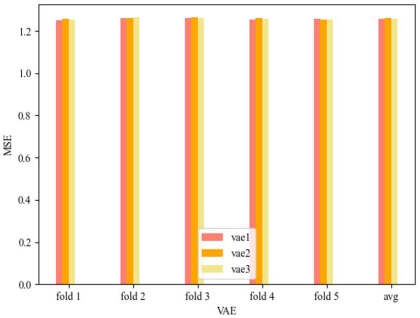
Figure 4. MSE of VAE.

The VAE models for the three convolutional kernel cases can be seen in Figure 4. vae1 in Figure 4 represents the Test MSE for the VAE model with convolutional kernel of Wang et al. (2024) and Liang et al. (2021) is 1.257207727, vae2 represents the Test MSE for convolutional kernel of Liang et al. (2021) and Chong et al. (2021) is 1.259705973, and vae3 represents the Test MSE for convolutional kernel of Chong et al. (2021) and Mir et al. (2024) is 1.257824469. The smallest MSE is 1.257207727 when the number of convolutional kernels is (Wang et al., 2024; Liang et al., 2021). The maximum MSE is 1.259705973 when the number of convolution kernels is (Liang et al., 2021; Chong et al., 2021). The range of model MSE is during the range of [1.2572, 1.2597].

To compare with the WCOS model proposed in this paper, the root mean square error obtained by combining the VAE model with wavelet variations, a one-dimensional support vector machine, and using the five-fold method is shown below.

Figure 5 represents the MSE of WR-VAE-OCSVM for the six convolutional kernel cases, and the Test MSE of the VAE model with the convolutional kernel of Wang et al. (2024) and Liang et al. (2021) is 1.257626295, that of the convolutional kernel of Liang et al. (2021) and Chong et al. (2021) is 1.257779431, that of the convolutional kernel of Chong et al. (2021) and Mir et al. (2024) is 1.258005643, that of the convolutional kernel for Mir et al. (2024) and Li et al. (2024) has a Test MSE of 1.256320214, the Test MSE for convolution kernel for [32, 64] has a Test MSE of 1.256026459, and the Test MSE for convolution kernel for [64, 128] has a Test MSE of 1.259554124, and it can be seen that the model error is minimized at convolution kernel for [32, 64], when the Test MSE is 1.256026459, and when the convolution kernel is [64, 128], the model error is the largest, at this time the Test MSE is 1.259554124, and the error range is in [1.256026459, 1.259554124].

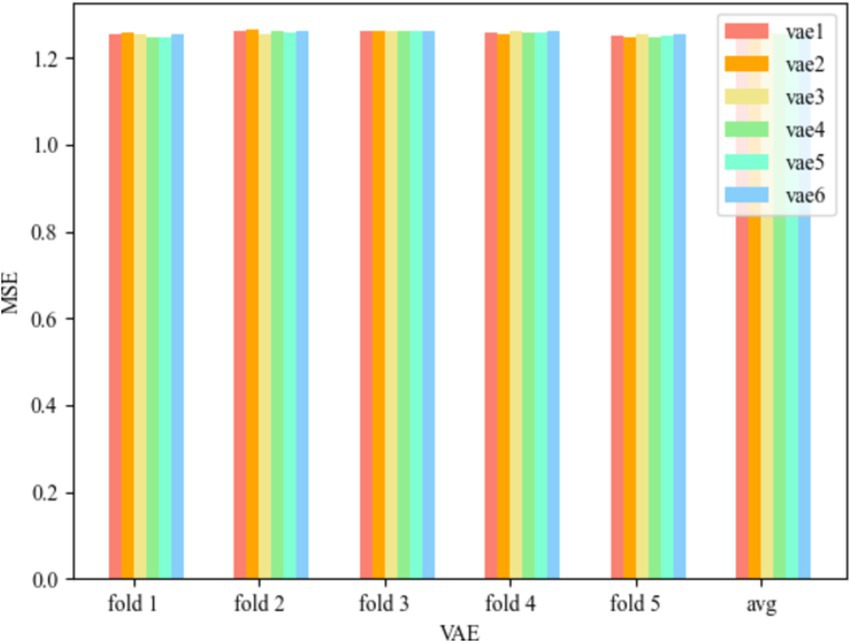
Figure 5. MSE of WR-VAE-OCSVM.

Figure 6 represents the MSE of WR-CAE-OCSVM for the six convolution kernel cases, and the Test MSE of the VAE model with convolution kernel (Wang et al., 2024; Liang et al., 2021) is 1.076472855, the Test MSE with convolution kernel (Liang et al., 2021; Chong et al., 2021) is 1.055950403, the Test MSE with convolution kernel (Chong et al., 2021; Mir et al., 2024) is 1.048900998, and the Test MSE of the VAE model with convolution kernel [16, 32] is 1.034770775, Test MSE for convolution kernel of [32, 64] is 1.012387657, and Test MSE for convolution kernel of [64, 128] is 1.007082856, which can be seen that the model error is minimum when the convolution kernel is [64, 128], and at this time Test MSE is 1.007082856, and the model error is maximum when the convolution kernel is (Wang et al., 2024; Liang et al., 2021), which is 1.007082856. At this time, the Test MSE is 1.076472855, and the error range is [1.007082856, 1.076472855].

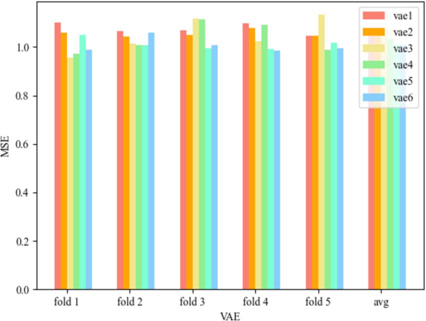
Figure 6. MSE of WR-CAE-OCSVM.

Comparing the two models, it is obvious that the error of the model proposed in this paper is much lower than that of WR-VAE-OCSVM, and compared with the WR-VAE-OCSVM model, the minimum error is lower by 0.248944, which reduces it by 19.82%, and the accuracy of the WCOS model still performs better in a variety of test rounds, which verifies the validity and advancement of the model. To improve the detection accuracy of the model, the subsequent content will discuss the effects of hyperparameters in the model and find the optimal parameters, respectively.

4.3.2 Hyperparameter determination

The modules that need to determine hyperparameters include the OCSVM module and the convolutional autoencoder module. The hyperparameters that the OCSVM module needs to determine are the control factor C and the kernel function k. Control factor Select C = 1 × 10−4, 1 × 10−3, 5 × 10−3, 1 × 10−2, 5 × 10−2 and 1 × 10−1 performance. Commonly used kernel function is linear function, polynomial function, radial basis function, the sigmoid function, formula by khihj=φhiTφhj is given by Equation 14:

klinehihj=hiThjkpolyhihj=a1hiThj+b1dkrbfhihj=exp−hi−hj2σ2ksigmoidhihj=tanha2hiThj+b2    (14)

Where a1 and b1 are polynomial coefficients, σ are width parameters, and a2 and b2 are coefficients of the sigmoid function. What the convolutional self-coder module needs to determine is the convolutional kernel i and j. This article arranged the 6 kinds of combinations, respectively (I = 2, j = 4), (I = 4, j = 8), (I = 8, j = 16), (I = 16, j = 32), (I = 32, j = 64), (I = 64, j = 128). The results of each model are as follows.

For the control group OCSVM, Figure 7 shows that the AUC value of the OCSVM model is higher only when the kernel function k = krbf. When the kernel functions k = klinear, k = kpoly, and ksigmoid, the AUC values of the OCSVM model are lower. When the kernel function k = krbf, the AUC value is less affected by the control factor C. When k = krbf and C = 1 × 10–4, the OCSVM model achieved the best performance in this task (AUC = 0.855).

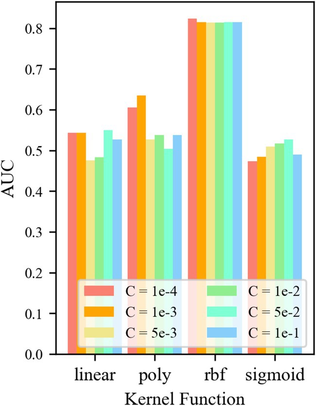
Figure 7. AUC at different parameters.

For control group No. 2 TF24-OCSVM, Figure 8 shows that when kernel functions k = krbf and klinear, the AUC value of the TF24-OCSVM model is higher. When the kernel functions k = kpoly and ksigmoid, the AUC value of the TF24-OCSVM model is low. When the kernel function k = krbf, the AUC value is less affected by the control factor C. When the kernel function k = klinear, the AUC value has a greater influence on the control factor C. When k = klinear and C = 1 × 10−4, the TF24-OCSVM model in this task achieved the best performance (AUC = 0.716).

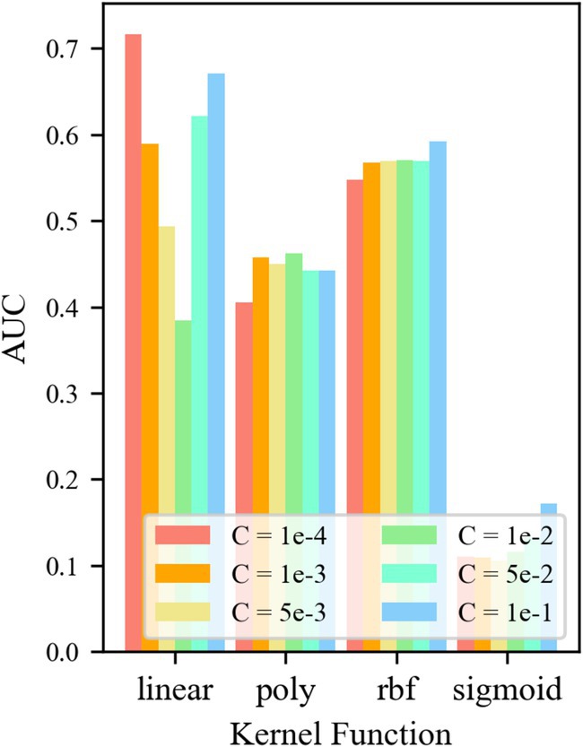
Figure 8. AUC for different parameters of TF24-OCSVM.

For the control group No. 3 CAE-OCSVM, the results are shown in Figure 9. Figure 9 shows that when k = krbf, the AUC of the CAE-OCSVM model is significantly higher than the AUC of k = klinear, kpoly, and ksigmoid. Therefore, the kernel function of the CAE-OCSVM model is set to krbf. In this case, when the kernel is 2–4, the maximum AUC is 0.736 (C = 1 × 10−3). When the kernel is 4–8, the maximum AUC is 0.867 (C = 1 × 10−3). When the kernel is 8–16, the maximum AUC is 0.841 (C = 1 × 10−3)). When the Kernel is 16–32, the maximum AUC is 0.842 (C = 5 × 10−2). When the kernel number is 32–64, the maximum AUC is 0.846 (C = 1 × 10−3). When the kernel is 86–128, the maximum AUC is 0.852 (C = 1 × 10−3). Therefore, to achieve the best performance of the CAE-OCSVM model in this task, the kernel function is set to k = krbf, the convolution kernel is set to 4–8, and the control factor is set to C = 1 × 10−3.

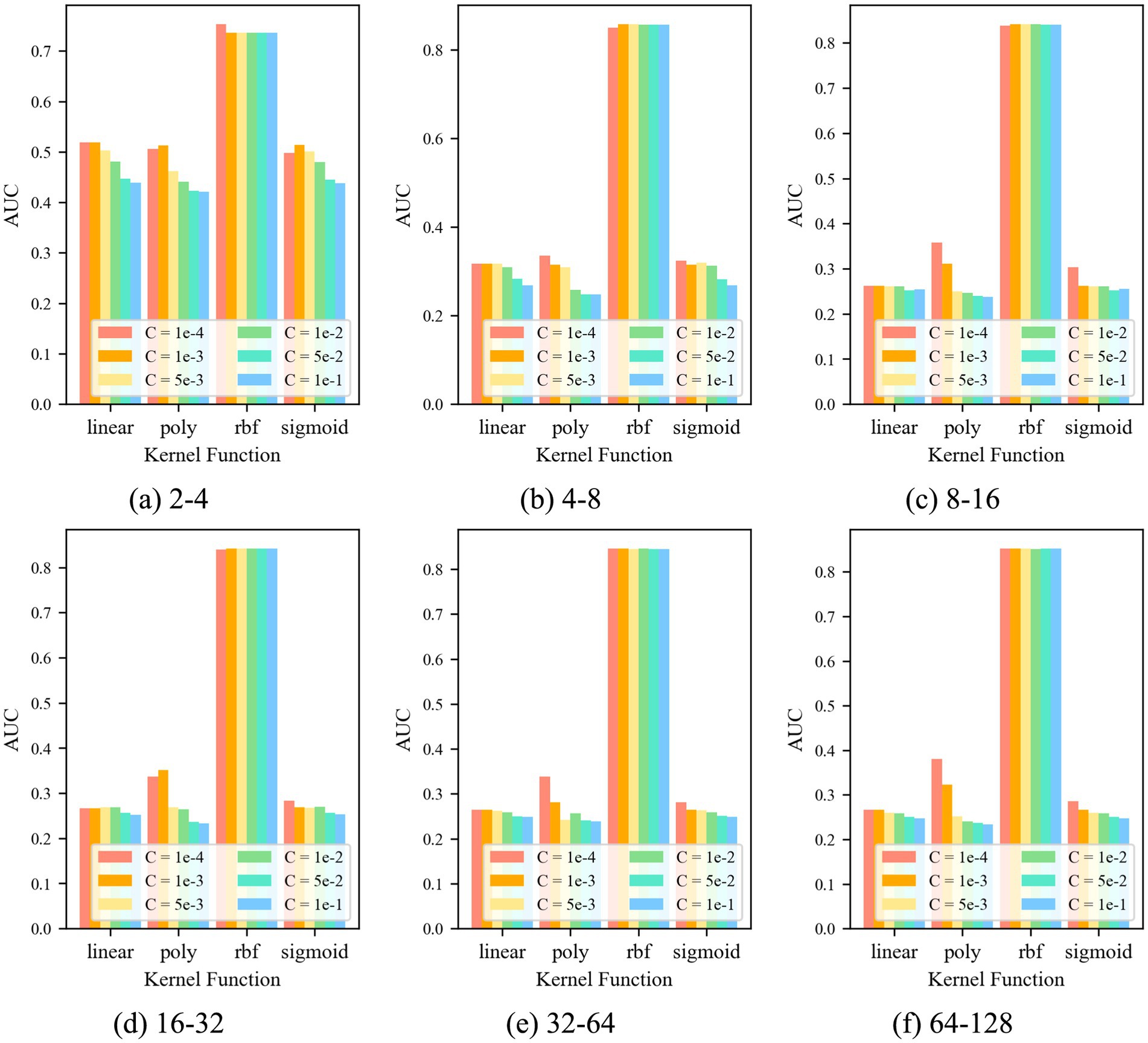
Figure 9. AUC of CAE-OCSVM with different parameters.

For control group No. 4 WR-OCSVM, the results are shown in Figure 10. Figure 10 shows that when kernel function k = krbf, the minimum AUC value of the WR-OCSVM model reaches 0.814. When the kernel function k = klinear, the maximum AUC of the WR-OCSVM model reaches 0.538. When the kernel function k = kpoly, the maximum AUC value of the WR-OCSVM model reaches 0.601. When the kernel function k = ksigmoid, the maximum AUC value of the WR-OCSVM model reaches 0.526. Therefore, when the kernel function k = krbf, the lowest AUC value is significantly higher than the highest AUC value when the kernel function k = klinear、kpoly、ksigmoid. When the kernel function k = krbf and the control factor C = 1 × 10−4, the AUC value is the highest, reaching 0.824. Therefore, to achieve the best performance of the WR-OCSVM model in this task, the kernel function is set to k = krbf, and the control factor is set to C = 1 × 10−4.

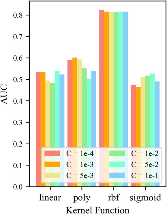
Figure 10. AUC at different parameters.

For the control group No. 5 WR-TF24-OCSVM, the results are shown in Figure 11. It is shown that when the kernel functions k = krbf and klinear, the AUC value of the TF24-OCSVM model is higher. When the kernel functions k = kpoly and ksigmoid, the AUC value of the TF24-OCSVM model is low. When the kernel function k = krbf, the AUC value is less affected by the control factor C. When the kernel function k = klinear, the AUC value is greatly affected by the control factor C. When k = klinear and C = 1 × 10−4, the TF24-OCSVM model in this task achieved the best performance (AUC = 0.796).

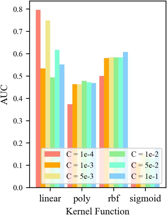
Figure 11. AUC at different parameters.

For the control group No. 6 WR-CAE-OCSVM, the results are shown in Figure 12: when k = krbf, the AUC of the WR-CAE-OCSVM model is significantly higher than that when k = klinear, kpoly, and ksigmoid. Therefore, the kernel function of the WR-CAE-OCSVM model is set to krbf. In this case, when the kernel is 2–4, the maximum AUC is 0.779 (C = 1 × 10−3). When the kernel is 4–8, the maximum AUC is 0.822 (C = 1 × 10−4). When the kernel is 8–16, the maximum AUC is 0.848 (C = 1 × 10−3). When the kernel is 16–32, the maximum AUC is 0.850 (C = 1 × 10−2). When the kernel is 32–64, the maximum AUC is 0.851 (C = 1 × 103). When the kernel is 86–128, the maximum AUC is 0.870 (C = 1 × 10−3). Therefore, to achieve the best performance of the WRCAE-OCSVM model in this task, the kernel function is set to k = krbf, the convolutional kernel is set to 64–128, and the control factor is set to C = 1 × 10−3.

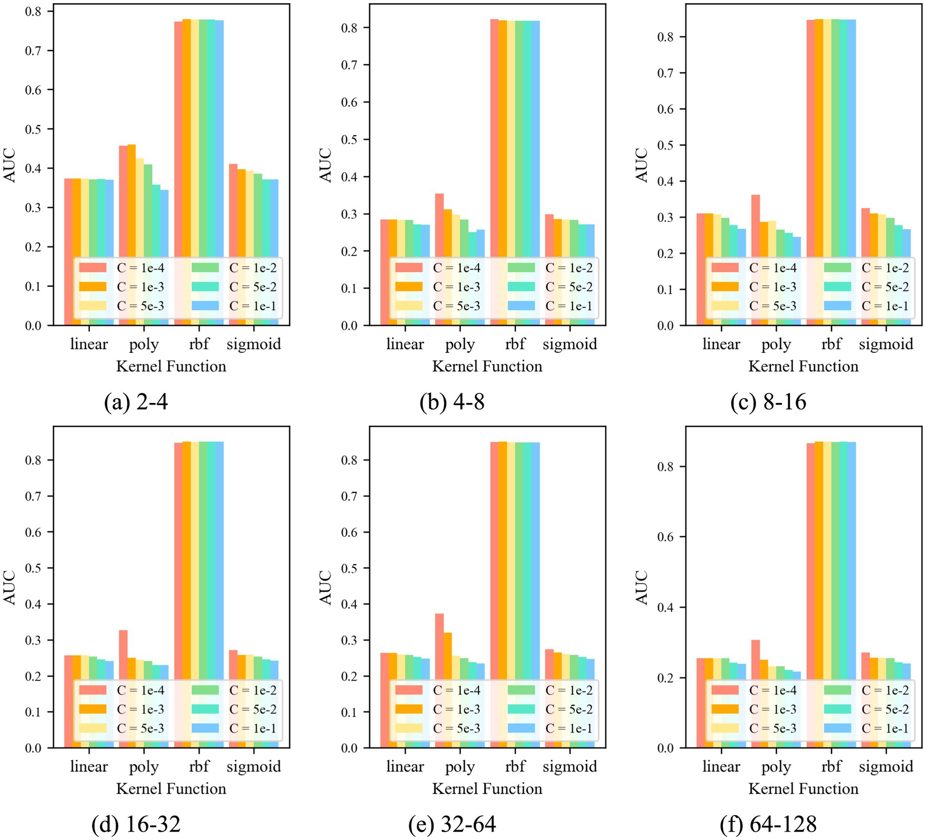
Figure 12. AUC at different parameters.

In summary, the optimal hyperparameter Settings of the six groups of models are shown in Table 2.

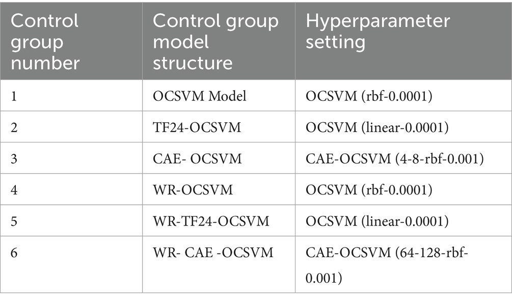
Table 2. Hyperparameter setting.

The table comprehensively shows the optimal hyperparameter settings of the six groups of models. The models are carefully tuned for different model structural characteristics, such as the OCSVM model kernel function is set to k = krbf and the control factor C = 0.0001 in control group 1, the kernel function is set to k = klinear and the control factor C = 0.0001 in control group 2, and the convolutional kernel is set to Liang et al. (2021) and Chong et al. (2021) for the CAE-OCSVM model in control group 3, the kernel function is set to Liang et al. (2021) and Chong et al. (2021), and the control factor C = 0.0001 in control group 4. the kernel function is set to k = krbf, control factor C = 0.0001, as in control group 4 WR-OCSVM model kernel function is set to k = krbf, control factor C = 0.0001, as in control group 5 WR-TF24-OCSVM model kernel function is set to k = klinear, control factor C = 0.0001, as in control group 6 WR- CAE -OCSVM model convolution kernel is set to [64, 128], the kernel function is set to k = krbf, control factor C = 0.0001.

4.3.3 Effectiveness of the developed framework

This paper established five groups of comparison experiments based on the cross-difference verification method to verify the validity. To remove the randomness of the neural network, each experiment was repeated 10 times. The experimental results are shown in Figure 13.

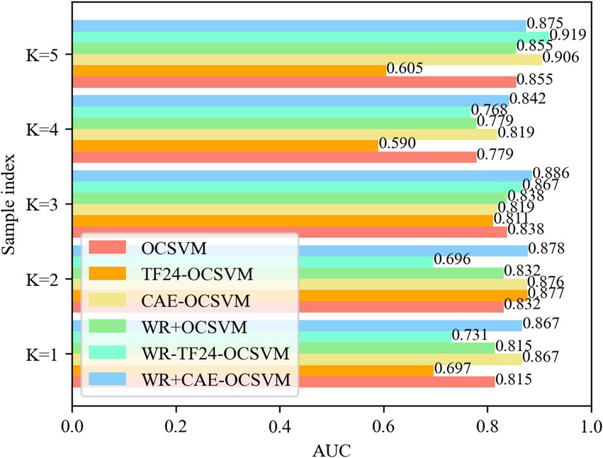
Figure 13. AUC for five-fold cross validation.

Figure 13 compares the AUC values of samples of six models OCSVM, TF24-OCSVM, CAE-OCSVM, WR-OCSVM, WR-TF24OCSVM, and WR-CAE-OCSVM under the best hyperparameters. It shows that the WR-CAE OCSVM has the highest AUC value in the samples with K = 1, 2, 3, and 4, reaching 0.867, 0.878, 0.886, 0.842, and 0.875, respectively.

Table 3 shows the Statistics of the mean, standard deviation, and variance of AUC of OCSVM, TF24-OCSVM, CAE-OCSVM, WR-OCSVM, WR-TF24-OCSVM and WR-CAE-OCSVM models, respectively.

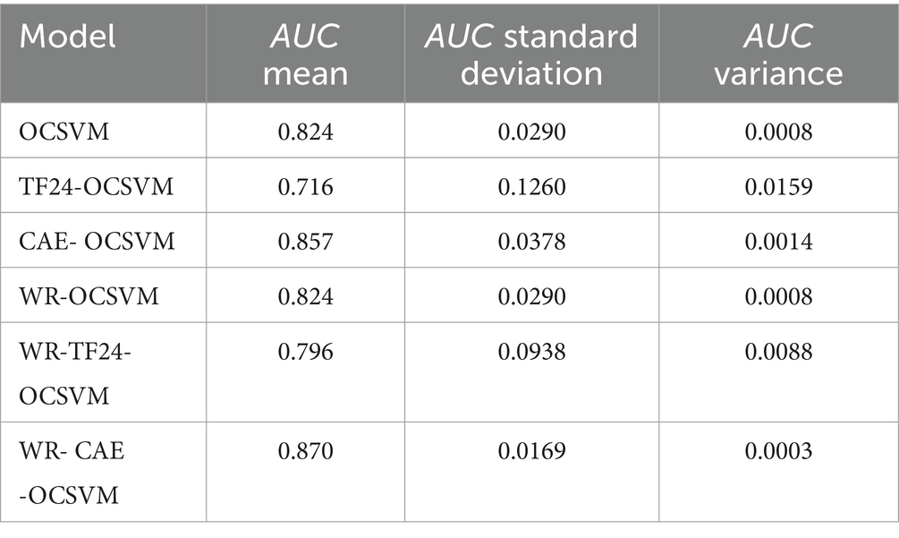
Table 3. Mean, standard deviation, and variance of AUC for 6 models.

Table 3 shows that the average AUC of WR-CAE-OCSVM is higher than that of WR-TF24-OCSVM (0.870–0.796)/ 0.870 × 100% = 8%. Similarly, the average AUC of WR-CAE-OCSVM is 5, 1, 18, and 5% higher than that of WR-OCSVM, CAE-OCSVM, TF24-OCSVM, and OCSVM, respectively. The above data reflect that WR-CAE-OCSVM has the best effect in this heart sound classification task.

Table 3 also shows that the AUC standard deviation of WR-CAE-OCSVM is lower than that of WR-TF24-OCSVM (0.0938–0.0169)/ 0.0938 × 100% = 82%. Similarly, the AUC standard deviation of WR-CAE-OCSVM is 42, 55, 87, and 42% lower than that of WROCSVM, CAE-OCSVM, TF24-OCSVM, and OCSVM, respectively. The AUC variance of WR-CAE-OCSVM is 97, 66, 80, 98, and 66% lower than that of WR-TF24-OCSVM, WR-OCSVM, CAE-OCSVM, TF24-OCSVM, and OCSVM, respectively. The above data reflect that the WR-CAE-OCSVM model has the best stability in this heart sound classification task.

4.3.4 Anti-noise ability of the developed framework

To verify the anti-noise ability of the WR-CAE-OCSVM model in the classification of heart sounds, four groups of experiments were carried out, respectively. In the experiment, Gaussian noise with different standard variance (sigma) was added to heart sounds to simulate ambient noise. As shown in Figure 14, gaussian noise with four different sigma values is set.

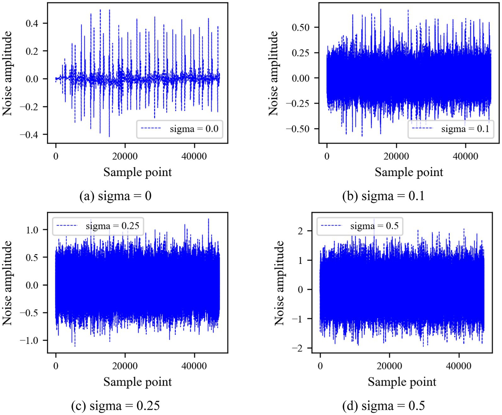
Figure 14. Four Gaussian noises with different sigma values.

Five groups of experiments were established based on the cross-difference verification method, and four groups of noise were added to each group of experimental data. To eliminate the randomness of the neural network, each experiment was repeated 10 times, and the experimental results are shown in Figure 15.

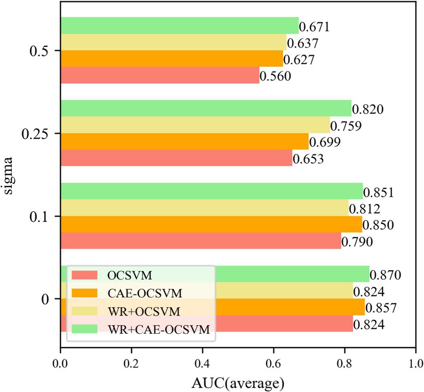
Figure 15. Sigma = 0, 0.1, 0.25, 0.5 anti-noise training AUC.

Figure 15 shows that the WR-CAE-OCSVM has the best classification effect in this task. When the noise of sigma = 0, the mean AUC of WR-CAE-OCSVM is higher than that of WR-OCSVM (0.870–0.824)/ 0.870 × 100% = 5.3%. The mean AUC of WR-CAE-OCSVM was 1.4 and 5.3% higher than that of CAE-OCSVM and OCSVM, respectively. When noise with sigma = 0.1, the mean AUC of the WR-CAE-OCSVM is 4.6, 0.2, and 7.2% higher than that of WR-OCSVM, CAEOCSVM and OCSVM, respectively. When noise with sigma = 0.25, the mean AUC of the WR-CAE-OCSVM is 7.4, 14.7, and 20.3% higher than that of WR-OCSVM, CAE-OCSVM and OCSVM, respectively. When noise with sigma = 0.5, the mean AUC of the WR-CAE-OCSVM is 5.0, 6.6, and 16.5% higher than that of WR-OCSVM, CAE-OCSVM, and OCSVM, respectively. To verify the stability of each model, Figure 16 shows the standard deviation of the AUC obtained from fi