In this section we investigate the following questions (which are essentially due to Klaus Fredenhagen): as we will see, the global transformation \((\mathcal _a)_\) corresponding to the extended local gauge transformation \(\partial _X\) (3.16) is a classical symmetry (i.e., the total Lagrangian is invariant). In which sense does the pertinent Noether current \(j^\mu (g;x)\) agree with the non-Abelian gauge current \(J^\mu (x)\) (3.29)? A main advantage of the global transformation over the local one is that the Lie algebra underlying \((\mathcal _a)\) is the Lie algebra of a compact Lie group; hence, the Haar measure (on this group) is available. By using that measure, it is possible to symmetrize the R- (or T-) product w.r.t. this group, such that this product commutes with \(\mathcal _a\) (Prop. 7.1). What are the consequences of this result for the possible anomaly of the conservation of the interacting quantum current \((j^\mu (g;x))_(g)}\) without assuming \(x\in g^(1)^\circ \) (Prop. 7.2)?

Global Transformation and Pertinent Classical Noether Current \(j^\mu \). We study the global, infinitesimal field transformation corresponding to \(\partial _X\), that is, in \(X(x)=X_b(x)t_b\in \textrm\mathfrak _c\) we replace \(X_b(x)\) by \(\delta _\).Footnote 29 This yields

(7.1)

Inserting the explicit formula (3.25) for \(\mathcal _a(x)\), we recognize that the first term, i.e., the contribution of the infinitesimal field shift to \(\partial _X^A\), does not contribute since the integration runs only over the support of F (which is compact). Therefore, \(\mathcal _a\) is solely a \(\textrm\mathfrak \)-rotation:

$$\begin \mathcal _a(F)=\,&\,-\kappa \int dx\,\Bigl (\Bigl [A^\mu (x),\frac\Bigr ]_a +\Bigl [u(x),\frac\Bigr ]_a+\Bigl [}(x),\frac}(x)}\Bigr ]_a\Bigr )\nonumber \\ =\,&\,-\kappa \int dx\,\Bigl ([t_a,A^\mu (x)]_b\frac +t_a,u(x)]_b\frac+[t_a,}(x)]_b\frac}_b(x)}\Bigr )\nonumber \\ =\,&\,-\kappa \,s_a(F) \end$$

(7.2)

with \(s_a\) defined in (3.5). Note that \(\omega _0\circ \mathcal _a=0\) with \(\omega _0\) being the vacuum state (2.15). To wit, for all basic fields \(\varphi \) it holds that \(\omega _0\bigl ([t_a,\varphi (x)]\cdot \frac\bigr )=\omega _0([t_a,\varphi (x)])\cdot \omega _0\bigl (\frac\bigr )\) and \(\omega _0([t_a,\varphi (x)])=0\). We also point out that

(7.3)

To wit, using the relations \([\partial _X,\partial _Y]=\kappa \,\partial _\) (3.37) and

$$\begin \partial _=\int dxdy\,\,\delta (x-y)\,X_a(x)Y_b(y)\,f_\,\mathcal _c(x) \end$$

and going over to the corresponding global transformations in the former relation (as explained before (7.1)), we obtainFootnote 30

$$\begin \mathcal _a,\mathcal _b]=\kappa \,f_\,\mathcal _c\ ,\quad \hbox \quad [\mathcal _,\mathcal _]=\kappa \,\mathcal _\ . \end$$

(7.4)

Obviously, \(\mathcal _a\) is a derivation w.r.t. the classical product and, due to \(\frac=\partial _\nu ^x\Bigl (\frac\Bigr )\), \( \varphi =A^\mu _a,u_a,}_a\), it holds that

$$\begin \mathcal _a\bigl (\partial ^\mu B(x)\bigr )=\partial ^\mu _x\,\mathcal _a\bigl (B(x)\bigr )\quad \hbox \quad B\in \mathcal . \end$$

(7.5)

That \(\mathcal _a\) is a derivation also with respect to the star-product (2.16) relies on the cancelations appearing in the commutator

$$\begin&\mathcal \,,\,\mathcal _a\otimes \textrm+\textrm\otimes \mathcal _a]=\kappa \int dx\,dy\,\Bigl (D^_\lambda (x-y)\, \frac^\mu (x)}\otimes \frac\nonumber \\&+D^+(x-y)\Bigl (-\frac\otimes \frac}_c(y)}+\frac}_b(x)}\otimes \frac\Bigr )\Bigr ) \cdot (f_+f_)=0\ ; \end$$

(7.6)

hence, we obtain

$$\begin \mathcal _a(F\star G)=&\,\mathcal _a\circ \mathcal \circ e^}(F\otimes G)=\mathcal \circ (\mathcal _a\otimes \textrm+\textrm\otimes \mathcal _a)\circ e^}(F\otimes G)\nonumber \\ =&\,\mathcal \circ e^}\bigl (\mathcal _a(F)\otimes G+F\otimes \mathcal _a(G)\bigr )=\mathcal _a(F)\star G+F\star \mathcal _a(G)\ . \end$$

(7.7)

In (3.10)–(3.12) we already verified that

$$\begin \mathcal _a\bigl (L_\textrm(g;x)\bigr )=0\ ,\quad \mathcal _a\bigl (L_\textrm(g;x)\bigr )=0\ ,\quad \mathcal _a\bigl (L_\textrm(g;x)\bigr )=0 \end$$

(7.8)

(remember \(\mathcal _a=-\kappa \,s_a\)); hence, the total Lagrangian \(L(g;x)=L_\textrm(g;x)+L_\textrm(g;x)+L_\textrm(g;x)\) is invariant. At this stage, \(F^\) and \(D^\mu \) contain the switching function g; hence, this holds also for the Lagrangians; we indicate this by writing \(L(g;\bullet )\). We derive the pertinent classical Noether current \(j^\mu _a\) in the usual way (cf. e.g., [20, Chap. 4.2.3]):

$$\begin 0= &\mathcal _a\bigl (L(g;x)\bigr )=\sum _k \mathcal _a\bigl (\varphi _k(x)\bigr )\cdot \frac(x)+ \mathcal _a\bigl (\partial _\mu \varphi _k(x)\bigr )\cdot \frac(x) \nonumber \\ = &\partial ^x_\mu \sum _k\Bigl (\mathcal _a\bigl (\varphi _k(x)\bigr )\cdot \frac(x)\Bigr ) +\sum _k \mathcal _a\bigl (\varphi _k(x)\bigr )\cdot \Bigl [\frac(x)- \partial _\mu \frac(x)\Bigr ]\ , \end$$

(7.9)

where the sum over k is the sum over \(\varphi _k=A_b^\mu ,\,u_b,\,}_b\). Therefore, in classical field theory the interacting field belonging to the Noether current

$$\begin j_a^\mu (g;x):=-\Bigl (\mathcal _a\bigl (A^\nu _b(x)\bigr )\frac(x) +\mathcal _a\bigl (u_b(x)\bigr )\frac(x)+ \mathcal _a\bigl (}_b(x)\bigr )\frac}_b)}(x)\Bigr )\nonumber \\ \end$$

(7.10)

is conserved modulo the interacting field equations. (Note that (7.9) and (7.10) are equations for field polynomials with coefficients containing the function g.) In terms of the perturbative, classical, retarded fields (4.33) this result readsFootnote 31

$$\begin \partial _\mu ^x j_a^\mu (g;x)^\textrm_(g),0}=0\ . \end$$

(7.11)

Computing \(j^\mu (g;x):=j^\mu _a(g;x)\,t_a\) for the model at hand, we obtain

$$\begin j^\mu (g;x)=\kappa \Bigl (-[A_\nu (x),F^(x)]+\lambda [(\partial A)(x),A^\mu (x)]-[\partial ^\mu }(x),u(x)]+ }(x),D^\mu u(x)]\Bigr );\nonumber \\ \end$$

(7.12)

this result differs from the non-Abelian gauge current \(J^\mu \) given in (3.29): the first and the third term do not appear in \(J^\mu \), and \(J^\mu \) has a term \(\lambda \square A^\mu \) which does not emerge in \(j^\mu \). Setting \(g(x)=0\), we obtain the corresponding current for the free theory,

$$\begin j^\mu (0;x)=\kappa \Bigl (&-[A_\nu (x),(\partial ^\mu A^\nu (x)-\partial ^\nu A^\mu (x))]+\lambda [(\partial A)(x),A^\mu (x)]\nonumber \\&-\partial ^\mu }(x),u(x)]+[}(x),\partial ^\mu u(x)]\Bigr ), \end$$

(7.13)

which is conserved modulo the free field equations, i.e.,

$$\begin \partial _\mu ^x j^\mu (0;x)_0=0\ . \end$$

(7.14)

In Which Sense Agrees \(j^\mu \) with the Non-Abelian Gauge Current \(J^\mu \)? This paragraph applies to both (perturbative) classical and quantum field theory; for the interacting currents we use the notation of pQFT. To study the difference \((J^\mu -j^\mu )\) we restrict to \(x\in g^(1)^\circ \) and we write \(j^\mu (x):=j^\mu (g;x)\) if (x, g) satisfies this assumption. The crucial point is that on-shell the difference \((J^\mu _,0}-j^\mu _,0})\) is a term whose divergence vanishes identically. To wit, by using the field equation (2.29),Footnote 32 the first term of \(J^\mu _,0}\) can be written as

$$\begin \lambda \square A^\mu _,0}(x)= &\square A^\mu _,0}(x)-(1-\lambda )\square A^\mu _,0}(x)\nonumber \\ = &(1-\lambda )\partial ^\mu \partial ^\nu (A_\nu )_,0}(x)+\kappa \Bigl (\partial ^x_\nu ([A^\nu (x),A^\mu (x)])_,0}\nonumber \\&-([A_\nu (x),F^(x)])_,0}-([\partial ^\mu }(x),u(x)])_,0}\Bigr )-(1-\lambda )\square A^\mu _,0}(x)\ . \end$$

(7.15)

Inserting this result we obtain

$$\begin J^\mu _,0}(x)-j^\mu _,0}(x) & =(1-\lambda )(\partial ^\mu \partial ^\nu -g^\square ) (A_\nu )_,0}(x)\nonumber \\ & \quad \ +\kappa \,\partial ^x_\nu ([A^\nu (x),A^\mu (x)])_,0}\ ; \end$$

(7.16)

obviously, the divergence \(\partial _\mu ^x\)[r.h.s. of (7.16)] vanishes identically, i.e., without restriction to \(\mathcal _0\). In pQFT the conclusion is that on-shell conservation of \(j^\mu \) and \(J^\mu \) is violated by the same anomaly term:

$$\begin \partial _\mu ^x\,j^\mu _,0}(x)=\partial _\mu ^x\,J^\mu _,0}(x)=\bigl (\Delta (x)(S_\textrm)\bigr )_,0} \quad \hbox \quad x\in g^(1)^\circ ,\nonumber \\ \end$$

(7.17)

where \(\Delta (x)(S_\textrm)=\Delta _a(x)(S_\textrm)\,t_a\).

How to Fulfill Invariance of the R-Product w.r.t. the Global Transformation, i.e., the Renormalization Condition \(\textrm\mathfrak \)-Covariance? A crucial advantage of \(\mathcal _a\) over \(\partial _X\) is that \(\mathcal _a\) is a global transformation. In addition, since the structure constants are totally antisymmetric and non-vanishing, the Killing form is negative definite. In detail, the Killing form is defined by

$$\begin \langle T_a,T_b\rangle :=\textrm(t_at_b)=\sum _f_f_ \end$$

(7.18)

(where \(\textrm(t_at_b)\) is the matrix-trace of the matrix product \(t_a\cdot t_b\)) and, by the assumed properties of the structure constants (see the beginning of Sect. 2), it holds that

$$\begin \langle T_a,T_a\rangle =-\sum _(f_)^2<0\ . \end$$

(7.19)

Since the Killing form is negative definite, \(\textrm\mathfrak \) is the Lie algebra of a semisimple compact Lie group \(\mathfrak \). Due to the compactness, the Haar measure is available. By using the latter a quite simple proof can be given of the following statement.

Proposition 7.1

In the inductive Epstein–Glaser construction of the sequence \((R_)_}\) (see [18] or [20, Chaps. 3.1,3.2]), the symmetry relation

$$\begin \mathcal _a\circ R_=R_\circ \sum _^(\textrm\otimes \cdots \otimes \mathcal _a\otimes \cdots \otimes \textrm)\quad \forall a \end$$

(7.20)

(where on the r.h.s. \(\mathcal _a\) is the kth factor) is a renormalization condition, which can be satisfied by a symmetrization, which maintains the validity of all other renormalization conditions.

Proof

That (7.20) is a renormalization condition is most easily seen by considering the analogous (and equivalent) relation for \(T_n\) and by proceeding by induction on n, following the inductive Epstein–Glaser construction of the sequence \((T_n)\) ( [22] or [20, Chap. 3.3]). The claim follows then from the above obtained result that \(\mathcal _a\) is a derivation w.r.t. the star product (7.7).

With that, in the inductive step \((n-1)\rightarrow n\), we know that (where \(\Delta _n:=\^n\,\big \vert \,x_1=\ldots =x_n\}\))Footnote 33 satisfies (7.20). Let \(T_n\) be an “admissible” extension of \(T_n^0\) to , i.e., an extension fulfilling all further renormalization conditions. We aim to construct a symmetrization \(T_n^\textrm\) of \(T_n\) which satisfies (7.20) and maintains all other renormalization conditions. We do this by means of the Haar measure. Since this is a measure on the Lie group (and not on the Lie algebra), we study the finite transformation belonging to \((\mathcal _a)_a\), more precisely,

$$\begin \mathfrak \equiv \mathfrak (\underline):=\exp (\underline\,\underline})\quad \hbox \quad \underline\,\underline}:=\sum _a\lambda _a\mathcal _a\ . \end$$

(7.21)

Defining

$$\begin V(\mathfrak )T_n:=\mathfrak \circ T_n\circ (\mathfrak ^)^\ , \end$$

(7.22)

the symmetrized extension must satisfy

$$\begin V(\mathfrak )T_n^\textrm=T_n^\textrm\ , \end$$

(7.23)

which is equivalent to the assertion (7.20) for \(T_n^\textrm\) in place of \(R_\). To verify this equivalence, first note that application of \(\frac\big \vert _=\underline}\) to \(\mathfrak \circ T_n^\textrm=T_n^\textrm\circ \mathfrak ^\) (7.23) yields (7.20) for \(T_n^\textrm\). The reversed conclusion is obtained by multiple application of (7.20):

$$\begin \exp&(\underline\,\underline})\,T_n^\textrm=\sum _^\infty \frac\,\underline})^j}\,T_n^\textrm\overset T_n^\textrm\circ \sum _^\infty \frac^(\textrm\otimes \cdots \otimes \underline\,\underline}\otimes \cdots \otimes \textrm)\Bigr )^j}\\ =&\,T_n^\textrm\circ \sum _^\infty \frac\sum _\frac\, (\underline\,\underline}\otimes \textrm\otimes \cdots \otimes \textrm)^\cdots (\textrm\otimes \cdots \otimes \textrm\otimes \underline\,\underline})^\\ =&\,T_n^\textrm\circ \sum _^\infty \frac\,\underline})^}\otimes \cdots \otimes \frac\,\underline})^}\\ =&\,T_n^\textrm\circ \Bigl (\exp \bigl (\underline\,\underline}\bigr )\Bigr )^\ , \end$$

where the multinomial theorem is used.

With that we can follow [18, App. D] or [20, Chap. 3.2.7]. Since (7.20) is a renormalization condition, we know that

$$\begin V(\mathfrak )T_n^0=T_n^0\ . \end$$

(7.24)

Due to \(V(\mathfrak _1\mathfrak _2)=V(\mathfrak _1)\circ V(\mathfrak _2)\), the map \(\mathfrak \mapsto V(\mathfrak )\) is a representation.

Let an admissible extension \(T_n\) of \(T_n^0\) be given. One verifies that \(V(\mathfrak )T_n\) is then also an admissible extension of \(V(\mathfrak )T_n^0=T_n^0\). Hence,

$$\begin L_n(\mathfrak ):=V(\mathfrak )T_n-T_n \end$$

(7.25)

is the difference of two admissible extensions, in particular it fulfills \(\,}}L_n(\mathfrak )\subset \Delta _n\). One straightforwardly verifies that the map \(\mathfrak \mapsto L_n(\mathfrak )\) satisfies the “cocycle” relation

$$\begin L_n(\mathfrak _1\mathfrak _2)=V(\mathfrak _1)\circ L_n(\mathfrak _2)+L_n(\mathfrak _1) \ . \end$$

(7.26)

We are searching an \(L_n^\textrm\) such that \(T_n^\textrm:=T_n+L_n^\textrm\) is an admissible extension of \(T_n^0\) (in particular, it must hold that \(\,}}L_n^\textrm\subset \Delta _n\)) and that \(T_n+L_n^\textrm\) is invariant,

$$\begin T_n+L_n^\textrm\oversetV(\mathfrak )\bigl (T_n+L_n^\textrm\bigr )=L_n(\mathfrak )+T_n+V(\mathfrak )L_n^\textrm\ , \end$$

(7.27)

which is equivalent to

$$\begin L_n(\mathfrak )=L_n^\textrm-V(\mathfrak )L^\textrm_n\ . \end$$

(7.28)

We claim that \(L_n^\textrm\) is obtained by the symmetrization

$$\begin L_n^\textrm:=\int __0}d\mathfrak \,\,L_n(\mathfrak )\ , \end$$

(7.29)

where \(\mathfrak _0\) is the connected component of the unit \(\textbf=\mathfrak (\underline)\in \mathfrak \) and \(d\mathfrak \) is the Haar measure, that is, the uniquely determined measure on \(\mathfrak _0\) which is invariant under left- and right-translations (i.e., \(d(\mathfrak \mathfrak )=d\mathfrak =d(\mathfrak \mathfrak )\) for \(\mathfrak \in \mathfrak _0\)) and has norm 1 (i.e., \(\int __0}d\mathfrak =\textbf\)). We have to verify that \(L_n^\textrm\) (given by (7.29)) satisfies (7.28):

$$\begin L_n^\textrm-V(\mathfrak )L^\textrm_n\overset &\int __0} d\mathfrak \,\bigl (L_n(\mathfrak )-V(\mathfrak )\circ L_n(\mathfrak )\bigr )\\ \overset &\int __0} d\mathfrak \,\bigl (L_n(\mathfrak )-L_n(\mathfrak \mathfrak )+L_n(\mathfrak )\bigr )\\ = &\int __0} d\mathfrak \,L_n(\mathfrak )-\int __0} d(\mathfrak \mathfrak )\,L_n(\mathfrak \mathfrak )+\Bigl (\int __0} d\mathfrak \Bigr )\,L_n(\mathfrak )\\ = &L_n(\mathfrak )\ . \end$$

That \(T_n^\textrm=T_n+L_n^\textrm\) is an admissible extension of \(T_n^0\) is a consequence of (7.29) and the (above obtained) result that \(T_n+L_n(\mathfrak )\) is an admissible extension of \(T_n^0\) for all \(\mathfrak \in \mathfrak _0\).

\(\square \)

The Possible Anomaly of \(\partial _\mu ^x\,j^\mu (g;x)_,0}\) Without Assuming \(x\in g^(1)^\circ \). In the remainder of this section, we study conservation of \(j^\mu (g;x)_,0}\) for general (g; x). Inserting (7.10) into (7.9) we obtain

$$\begin \partial _\mu ^x\,j^\mu (g;x)=\sum _k\mathcal _a\bigl (\varphi _k(x)\bigr )\cdot \frac(g)\bigr )}\ , \end$$

(7.30)

where the sum over k is the sum over \(\varphi _k=A_b^\mu ,\,u_b,\,}_b\). (Similarly to (7.9)–(7.10) this is an equation for field polynomials.) Hence we can apply the theorem about the AMWI (given in [3, Sect. 5.2] or [20, Chap. 4.3], see also Theorem 4.1 and (4.21)): there exists a unique local functional

(7.31)

which satisfies certain properties (recalled in Theorem 4.1 for the case that the infinitesimal symmetry transformation is \(\partial _X\)): most important are the AMWI, whose on-shell version reads

$$\begin \partial _\mu ^x\,\bigl (j^\mu (g;x)\bigr )_(g),0}=\bigl (}(x)(S_\textrm(g))\bigr )_(g),0}\ , \end$$

(7.32)

and locality, see (4.15). Due to the latter, the map \(\Delta _a(x)(\bullet )\) introduced in (4.21) satisfies \(\Delta _a(x)\bigl (B(g)\bigr )=0\), if \(x\not \in \,}}g\). For the possible anomaly \(}(x)(S_\textrm(g))\) this means that

$$\begin }(x)(S_\textrm(g))=0\quad \hbox \quad x\not \in \,}}g. \end$$

(7.33)

Proposition 7.2

If the R-product commutes with the global transformation \(\mathcal _a\) (more precisely, (7.20) is satisfied), then it holds that

$$\begin \int dy \,\,\bigl (}(y)(S_\textrm(g))\bigr )_(g),0}=0\ . \end$$

(7.34)

The proof of this proposition uses the following result:

Lemma 7.3

It holds that

(7.35)

for any choice of \(c\in \mathbb \), where \([\bullet ,\bullet ]_\star \) denotes the commutator w.r.t. the on-shell star product (2.23).

Proof of Prop. 7.2. Let \(\mathcal \subset \mathbb \) be an open double cone containing \(\,}}g\), and let \(g_1\in \mathcal (\mathbb )\) be a test function which is equal to 1 on a neighborhood of \(\overline}\). With that and (7.32)–(7.33), (2.23) and the Bogoliubov formula (4.3), we may write

$$\begin \int dy\,\,\bigl (}(y)(&S_\textrm(g))\bigr )_(g),0}=\int dy\,\,g_1(y)\,\bigl (}(y)(S_\textrm(g))\bigr )_(g),0}\nonumber \\ = &-\overline\bigl (e_\otimes ^(g)/\hbar }\bigr )_0\star \int dy\,(\partial ^\mu g_1)(y)\, T\bigl (e_\otimes ^(g)/\hbar }\otimes j^\mu (g;y)\bigr )_0\ . \end$$

(7.36)

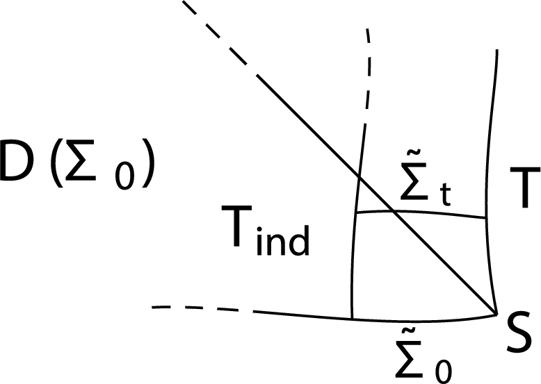
Fig. 1

Illustration of the proof of Prop. 7.2: double cone \(\mathcal \) containing \(\,}}g\) (with its past \(\mathcal +\overline_-\) and its future \(\mathcal +\overline_+\)) and respective supports of the (decomposed) test functions.

We decompose \(\partial ^ g_1=a^-b^\) such that \(\,}}a^\cap (\mathcal +\overline_-)=\emptyset \) and \(\,}}b^\cap (\mathcal +\overline_+)=\emptyset \). By causal factorization of the T-product and (2.23) and \(j^\mu (g;a^\mu )=j^(0;a_)\) (since \(\,}}g\cap \,}}a^\mu =\emptyset \)), and similarly for \(j^\mu (g;b^\mu )\), we obtain

$$\begin \int dy\,&(\partial ^\mu g_1)(y)\, T\bigl (e_\otimes ^(g)/\hbar }\otimes j^\mu (g;y)\bigr )_0\nonumber \\&=j^(0;a_)_0\star T\bigl (e_\otimes ^(g)/\hbar }\bigr )_0- T\bigl (e_\otimes ^(g)/\hbar }\bigr )_0\star j^(0;b_)_0\nonumber \\&=[j^(0;a_)_0\,,\,T\bigl (e_\otimes ^(g)/\hbar }\bigr )_0]_\star +T\bigl (e_\otimes ^(g)/\hbar }\bigr )_0\star j^(0;\partial _g)_0\ . \end$$

(7.37)

In the last term the second factor vanishes, due to (7.14). From Field independence of T we know that \(\,\,}}T\bigl (e_\otimes ^(g)/\hbar }\bigr )_0\subset }}\); therefore, we may vary \(a^\mu \) in the spacelike complement of \(\mathcal \) without affecting the remaining commutator in (7.37). Taking additionally into account that \(g_1\) is arbitrary (up to \(g_1\big \vert _}}=1\)), we may choose for \(a_\mu (y)\) a smooth approximation to \(-\delta _\,\delta (y^0-c)\), where \(c\in \mathbb \) is a sufficiently large constant:

$$\begin a_\mu (y)=-\delta _\,h(y^0)\quad \hbox \quad \int dy^0\,\, h(y^0)=1\ ,\quad h\in \mathcal ([c-\varepsilon ,c+\varepsilon ]) \end$$

for some \(\varepsilon >0\). Inserting this \(a^\mu \) into (7.37) and using Lemma 7.3, we get

$$\begin j^(0;a_)_0\,,\,T\bigl (e_\otimes ^(g)/\hbar }\bigr )_0]_\star = &-\int dy^0\,\,h(y^0)\int d\textbf\,\, j^0(0;(y^0,\textbf))_0\,,\,T\bigl (e_\otimes ^(g)/\hbar }\bigr )_0]_\star \\ = &-\Bigl (\int dy^0\,\,h(y^0)\Bigr )\int d\textbf\,\, j^0(0;(c,\textbf))_0\,,\,T\bigl (e_\otimes ^(g)/\hbar }\bigr )_0]_\star \\ = &-i\hbar \,\mathcal _a\Bigl (T\bigl (e_\otimes ^(g)/\hbar }\bigr )\Bigr )_0\ . \end$$

By the validity of (7.20) for \(T_n\) and by \(\mathcal _a\bigl (S_\textrm(g)\bigr )=0\) we obtain the assertion (7.34). \(\square \)

Proof of Lemma7.3. Due to spacelike commutativity the region of integration on the l.h.s. of (7.35) is a subset of

$$\begin \\,\big \vert \,(c,\textbf)\in \,}}F+(\overline_+\cup \overline_-)\,\}\ , \end$$

which is bounded for all \(c\in \mathbb \); therefore, this integral exists indeed. In addition, due to (7.14) and Gauss’ integral theorem, this integral does not depend on c. Hence, we may introduce the short notationFootnote 34

(7.38)

We first prove (7.35) for \(F=A_b^\rho (x)\): Inserting (7.13) and using \(A^\mu _a(y)\,,\,A^\rho _b(x)]_\star =-i\hbar \delta _\,D_\lambda ^(y-x)\) we obtain

$$\begin \int d^3y\,\,[j^0_a&(0;y)_0\,,\,A_b^\rho (x)_0]_\star =i\hbar \kappa \,f_\int d^3y\, \Bigl (\delta _\,\bigl (\partial ^0 A^\nu _d(y)-\partial ^\nu A^0_d(y)\bigr )\,D_^(y-x)\nonumber \\&+\delta _\,A_(y)_0\bigl (\partial ^0 D^_\lambda (y-x)-\partial ^\nu D^_\lambda (y-x)\bigr )\nonumber \\&-\delta _\,A_d^0(y)_0\,\lambda \,\partial _\mu D^_\lambda (y-x)-\delta _\,(\partial A_c)(y)_0\,\lambda \,D^_\lambda (y-x)\Bigr )\ . \end$$

(7.39)

Now we choose \(y^0=x^0\) in order that we may use the equal-time commutation relations (2.22). Hence, solely the commutators \([\partial ^0 A(x^0,\textbf),A(x)]_\star \sim \partial ^0\,D_\lambda (0,\textbf-\textbf)\sim \delta (\textbf-\textbf)\) contribute. By straightforward computation we obtain that the terms depending explicitly on \(\lambda \) cancel out and that

$$\begin \mathrm =-i\hbar \kappa \,f_\,A^\rho _c(x)_0=i\hbar \,\mathcal _a\bigl (A^\rho _b(x)\bigr )_0\ . \end$$

(7.40)

Proceeding analogously one verifies the assertion (7.35) for \(F=u(x)\) and \(F=}(x)\); this verification is even somewhat simpler than for \(F=A^\rho (x)\), because the free field equation is simpler.

Since \(\mathcal _a\) is a derivation w.r.t. the classical product, more precisely \(\mathcal _a(F\cdot G)_0=\mathcal _a(F)_0\cdot G_0+F_0\cdot \mathcal (G)_0\), it remains to prove that

$$\begin Q_0,\varphi ^1_(x_1)\cdot \ldots \cdot \varphi ^n_(x_n)]_\star =i\hbar \sum _^n\varphi ^1_(x_1)\cdot \ldots \cdot \mathcal _a\bigl (\varphi ^k_(x_k)\bigr )_0\cdot \ldots \cdot \varphi ^n_(x_n)\ ,\nonumber \\ \end$$

(7.41)

where \(\varphi ^k\in \}\}\). We proceed by induction on n. We have just verified the case \(n=1\), i.e., \(Q_0,\varphi _(x)]_\star =i\hbar \,\mathcal _a\bigl (\varphi _b(x)\bigr )_0=i\hbar \kappa \, f_\,\varphi _(x)\). In the step \(n\rightarrow n+1\) we use the relationFootnote 35

$$\begin \varphi ^1_&(x_1)\cdot \ldots \cdot \varphi ^_,0}(x_)=\bigl (\varphi ^1_(x_1)\cdot \ldots \cdot \varphi ^n_(x_n) \bigr )\star \varphi ^_,0}(x_)\nonumber \\&-\sum _^n\,}}(\pi _k)\,\bigl (\varphi ^1_(x_1)\cdot \ldots }\ldots \cdot \varphi ^n_(x_n)\bigr )\cdot \omega _0\bigl (\varphi ^k_(x_k)\star \varphi ^_,0}(x_)\bigr )\ , \end$$

(7.42)

where \(}\) means that the kth factor is omitted and \(\,}}(\pi _k)\) is the fermionic sign coming from the permutation \(\varphi ^1_(x_1)\cdot \ldots \cdot \varphi ^n_(x_n)\mapsto \varphi ^1_(x_1)\cdot \ldots }\ldots \cdot \varphi ^n_(x_n) \cdot \varphi ^k_(x_k)\). We also take into account that the commutator \([Q_0,\bullet ]_\star \) is a derivation w.r.t. the on-shell \(\star \)-product. With that we obtain

$$\begin \frac[Q_0,\,&\varphi ^1_(x_1)\cdot \ldots \cdot \varphi ^_,0}(x_)]_\star \nonumber \\ = &\sum _^n\bigl (\varphi ^1_(x_1)\cdot \ldots \cdot \mathcal _a\bigl (\varphi ^k_(x_k)\bigr )_0\cdot \ldots \cdot \varphi ^n_(x_n)\bigr ) \star \varphi ^_,0}(x_)\nonumber \\&+\bigl (\varphi ^1_(x_1)\cdot \ldots \cdot \varphi ^n_(x_n)\bigr )\star \mathcal _a\bigl (\varphi ^_}(x_)\bigr )_0 \nonumber \\&-\sum _^n\,}}(\pi _k)\,\sum _\bigl (\varphi ^1_(x_1)\cdot \ldots }\ldots \cdot \mathcal _a\bigl (\varphi ^j_(x_j)\bigr )_0\cdot \ldots \cdot \varphi ^n_(x_n)\bigr )\nonumber \\&\qquad \qquad \qquad \qquad \cdot \omega _0\bigl (\varphi ^k_(x_k)\star \varphi ^_,0}(x_)\bigr )\ . \end$$

(7.43)

Since it holds that

$$\begin \omega _0&\Bigl (\mathcal _a\bigl (\varphi ^k_(x_k)\bigr )_0\star \varphi ^_}(x_)_0\Bigr )+ \omega _0\Bigl (\varphi ^k_(x_k)_0\star \mathcal _a\bigl (\varphi ^_}(x_)\bigr )_0\Bigr )\\&\overset\omega _0\Bigl (\mathcal _a\bigl (\varphi ^k_(x_k)\star \varphi ^_}(x_)\bigr )_0\Bigr )=0 \end$$

(by using \(\omega _0\circ \mathcal _a=0\)), we may add

$$\begin 0= &-\sum _^n\,}}(\pi _k)\,\bigl (\varphi ^1_(x_1)\cdot \ldots }\ldots \cdot \varphi ^n_(x_n)\bigr )\\&\cdot \Bigl (\omega _0\bigl (\mathcal _a(\varphi ^k_(x_k))_0\star \varphi ^_}(x_)_0\bigr )+ \omega _0\bigl (\varphi ^k_(x_k)_0\star \mathcal _a(\varphi ^_}(x_))_0\bigr )\Bigr ) \end$$

to the right hand side of (7.43); using again (7.42) we see that the r.h.s of (7.43) is equal to the r.h.s. of the assertion (7.41) with \((n+1)\) in place of n.

\(\square \)

Remark 7.4

The situation is similar to spinor QED (see [14] or [20, Chap. 5.2]) and scalar QED (see [21]): In these models the global transformation is the charge number operator,

(7.44)

for spinor QED and \(\delta _:=\phi (x)\,\frac-\phi ^*(x)\,\frac\) for scalar QED. Proceeding similarly to (7.9)–(7.10), we see that the classical Noether current \(j^\mu (g;x)\) belonging to charge number conservation of the total Lagrangian, i.e., \(\theta \bigl (L_0(x)+L_\textrm(g;x))\bigr )=0\), satisfies also the relation (7.30) with \(\theta \) in place of \(\mathcal _a\),Footnote 36 explicitly

$$\begin & \partial _\mu j^\mu (g;x)=i\Bigl ( \frac\wedge \psi (x) -\overline(x)\wedge \frac(x)}\Bigr )\quad \hbox \quad \nonumber \\ & j^\mu (g;x)=\overline(x)\wedge \gamma ^\mu \psi (x)\ , \end$$

(7.45)

and for spinor QED, see the explanations concerning the current \(j^\mu (g;x)\) given at the end of this remark. Hence, for the on-shell AMWI belonging to the corresponding local transformation, i.e.,

$$\begin \delta _:=\int dx\,\,q(x)\,\delta _\quad \hbox \quad q\in \mathcal (\mathbb ) \quad \hbox \quad \end$$

(7.46)

we obtain also the anomalous current conservation (7.32), where, similarly to (7.32), the test function g switching the interaction is arbitrary. Proceeding analogously to the proof of Prop. 7.2, it is proved in these references that invariance of the R-product w.r.t. \(\theta \) (i.e., (7.20) with \(\theta \) in place of \(\mathcal _a\))Footnote 37   implies that the integral over the anomaly (of the current conservation) vanishes also in these models, i.e., (7.34) holds also there. However, to prove that the anomaly itself can be removed by finite, admissible renormalizations (without assuming \(x\in g^(1)^\circ \)) requires quite a lot of additional work, including an investigation of some classes of Feynman diagrams. For the Noether current \(j^\mu _,0}(x)\equiv j^\mu _,0}(g;x)\) belonging to \(\mathcal _a\) and for the non-Abelian gauge current \(J^\mu _,0}(x)\), both restricted to the region \(x\in g^(1)^\circ \) (see (7.17)), we have given a shorter and more elegant proof of the removability of the anomaly \((\Delta (x)(S_\textrm))_,0}\) (in Sect. 5) by using the consistency condition for the (possible) anomaly. Unfortunately, the anomaly consistency condition (5.1) is trivial (i.e., \(0=0\)) for spinor and scalar QED.

Note that for scalar QED the Noether current of the interacting theory isFootnote 38

$$\begin j^\mu (g;x)=i\bigl (\phi (x)\,(D^\mu \phi )^*(x)-\phi ^*(x)\,D^\mu \phi (x)\bigr )\quad \hbox \quad D^\mu _x:=\partial ^\mu _x+i\kappa g(x)\,A^\mu (x)\nonumber \\ \end$$

(7.47)

being the covariant derivative; hence, similarly to the situation in this paper, \(j^\mu (g;x)\) differs from the corresponding current of the free theory \( j^\mu (0;x)\). But in spinor QED there is the peculiarity that these two currents agree: \(j^\mu (g;x)=j^\mu (0;x)=\overline(x)\wedge \gamma ^\mu \psi (x)\), because \(L_\textrm(x)=j^\mu (0;x)\,A^\mu (x)\) satisfies \(\frac}=0=\frac})}\), see (7.10).