Diagrammatic Notations

We introduce some diagrammatic notations used in the computations of commutation relations of the algebra \(\mathscr _^\left( \epsilon _, \epsilon _\right) \). Let V be the N-dimensional vector space, which is the fundamental representation space of \(\textrm(N)\). We use the following diagrams to represent a tensor \(T^i_\cdots i_}_j_\cdots j_}\) in \(}^\otimes V^\):

In this diagram, we have m incoming lines and n outgoing lines. Contracting upper and lower indices are represented by connecting incoming and outgoing lines. We denote the generators of the algebra as \(Z^i_j\), \(}^i_j\), \(\lambda _a\), and \(}^a\) by the following diagrams:

All elements appearing in this paper can be expressed using diagrams, which consist of usual tensors (that commute with everything) decorated with white and black points on the oriented lines, along with , and at the endpoints of the oriented lines.

We envision every element in the diagram that consists of \(Z^i_j\), \(}^i_j\), \(\lambda _a\), \(}^a\) as having a vertical dashed line (serve as auxiliary lines) passing through it. Whenever we continuously move an element A around and cross such a vertical line going through another element B, there may be some quantum correction term proportional to \(\epsilon _\). This phenomenon arises from the non-commutativity of the matrix components (3.1). Diagrammatically, this phenomenon is illustrated in the following diagram, where we use a wavy line to denote quantum contractions:

These quantum corrections are generated by the canonical quantization conditions (3.1). Diagrammatically:

Let us illustrate how to apply the diagrammatic notation for performing calculations on the quantum algebra of the matrix model by considering two examples.

Example A.1

Let us demonstrate that \(\mu ^_\) generates the \(\mathfrak (N)\) action, as stated in Proposition (3.1), using our diagrammatic notation. The operator \(\mu ^i_j\) is depicted diagrammatically as:

Next, we show (3.3): \([\mu ^_,Z^_]=\epsilon _ \delta ^_Z^_-\epsilon _\delta ^_Z^_\) and (3.5) \([\mu ^_,\lambda _^]=-\epsilon _ \delta ^_ \lambda _^\) diagrammatically:

Example A.2

Another example is to show (5.2) in Proposition (5.3):

$$\operatorname \left( A\left[ Z, Z^\right] B\right) =\operatorname \left( A\left( \epsilon _-\lambda _ }}}^a\right) B\right) +\epsilon _ \operatorname A \operatorname B$$

diagrammatically. To show this, we consider the following identity:

Apply the following commutation relation (\(\mu ^i_j\) generates \(\mathfrak (N)\) action):

We have

On the other hand:

Combining A.7, A.8, we have

Connection to Murnaghan-Nakayama Rule

In this appendix, we establish connections between the terms:

$$\begin&C(n_,n_,\cdots ,n_):=\epsilon ^i_\cdots i_}(\lambda ^}^})_}(\lambda ^}^})_}\cdots (\lambda ^}^})_} \end$$

(B.1)

$$\begin&t_:=\textrm(}^) \end$$

(B.2)

to the Schur polynomials and power sum polynomials in N variables. We demonstrate that equation (5.43) is equivalent to the Murnaghan-Nakayama rule, which is a combinatorial rule governing the transformation between the bases of Schur polynomials and power sum polynomials within the ring of symmetric polynomials. Since equation (5.43) is derived using the diagrammatic method in this paper, this can be viewed as a new diagrammatic proof of the classical Murnaghan-Nakayama rule. For further details on the Murnaghan-Nakayama rule, we refer to [26, 27].

Following [4], one can view \(C(n_1,n_2,\cdots ,n_N)\) and \(\textrm(}^n)\) as polynomials in the variables \(\}^i_j, 1\le i,j \le N;}_i, 1 \le i \le N\}\). The connections between \(C(n_1,n_2,\cdots ,n_N)\) and \(\textrm(}^n)\) to the Shur polynomials and power sum polynomials are established by evaluating them on diagonal matrices \(Z^=diag(z_1,z_2,\cdots ,z_N)\). Consequently, \(C(n_1,n_2,\cdots ,n_N)\) and \(\textrm(}^n)\) becomes

$$\begin \det [z^}_]_\prod _^}_ \quad \text \quad \sum _^z_^ \end$$

(B.3)

We assume \(0 \le n_1< n_2< n_3< \cdots <n_N\). Let \(\mu _:=n_-(N-i)\), then \(\mu _1\ge \mu _2\ge \mu _3\ge \cdots \mu _N\ge 0\). Hence (B.3) becomes (up to an overall sign)

$$\begin \det [z^+N-i}_]_\prod _^}_ \quad \text \quad P_=\sum _^z_^ \end$$

(B.4)

where \(P_\) is the power sum polynomial. The classical definition of Schur polynomials states:

$$s_(z_1,z_2,\cdots ,z_N)=\frac+N-i}_]_}_]_}$$

Now, let us evaluate equation (5.43) at \(Z^=diag(z_1,z_2,\cdots ,z_N)\), and divide both sides by \(C(0,1,2,\cdots ,N-1)\). This yields an equation of the following form:

$$\begin P_(z_1,z_2\cdots ,z_N)s_(z_1,z_2,\cdots ,z_N)=\sum _\pm s_(z_1,z_2\cdots ,z_N) \end$$

(B.5)

Here, \(\Lambda \) represents a set of specific integer partitions. Let us identify the integer partitions \(\nu \in \Lambda \) that appear in the summation on the right-hand side of (B.5), along with the sign of each term. We illustrate this in terms of Young diagrams. We will consider two types of Young diagrams associated with \(C(n_1,n_2,\cdots ,n_N)\), where the condition \(0 \le n_1< n_2< n_3< \cdots <n_N\) do not need to be satisfied. The first kind of diagrams are the non-standard one: we simply place \(n_\) boxes on the ith row. We allow the number of boxes to be exchanged between two different rows, and after exchanging, we assign a negative sign. This reflects the totally antisymmetric property of \(C(n_1,n_2,\cdots ,n_N)\).

For example for \(N=5\), and C(1, 3, 8, 5, 7), we have the following (non-standard) Young diagram:

Let us illustrate how to obtain the second type of Young diagrams associated with \(C(n_1,n_2,\cdots ,n_N)\). These are the standard diagrams, each carrying a sign. We begin with the first type of Young diagram (typically non-standard) associated with \(C(n_1,n_2,\cdots ,n_N)\), which carries a sign. We rearrange the rows such that the number of boxes does not increase, and then we mark the first \(N-i\) boxes in each ith row with a cross. Each row exchange results in a minus sign. After removing all the crosses and shifting all the boxes to the leftmost position, we obtain the second tpye of Young diagram (a standard one) corresponding to a partition \(\nu \) and carrying a sign. By the correspondence described previously, \(C(n_1,n_2,\cdots ,n_N)\) corresponds to the Schur polynomial \(\pm s_\).

An example will best illustrate this. Consider the above example C(1, 3, 8, 5, 7):

In the following, let us identify the integer partitions corresponding to the terms on the right-hand side of equation (5.43) in terms of (standard) Young diagrams. It’s better to proceed by considering an example. Let us take \(n=5\) and \(C(n_1=1,n_2=3,n_3=5,n_4=7,n_5=8)\) in (5.43). There are 5 terms on the right hand side of equation (5.43). The first term is \(C(1+5,3,5,7,8)\), which corresponds to the following Young diagram of the second type:

In the above diagram, we decorate the newly added boxes with black dots. Now, we permute the number of boxes in each row until we arrive at a diagram with a non-increasing number of boxes in each row from top to bottom. This permutation is achieved by first exchanging the number of boxes in the 4th and the 5th rows, and then exchanging the 3rd and the 4th rows, and so on. These exchanges can be visualized by moving the boxes containing black dots:

Finally, by removing all the crosses and shifting all the boxes to the leftmost position, we obtain the standard diagram corresponding to the partition labeling the Schur polynomial corresponding to this pariticular term \(C(1+5,3,8,5,7)\) in \(\textrm(}^5)C(1,3,5,7,8)\):

The sign of this term is \(+\).

By examining several additional examples, it becomes evident that the newly introduced boxes (depicted as boxes containing black dots) typically take on the following shape:

This shape is commonly referred to as a border-strip diagram. More precisely:

Definition B.1

Let \(\nu \) be a standard Young diagram and \(\mu \) another standard Young diagram contained within \(\nu \). We denote \(\nu \backslash \mu \) as the set of boxes in the Young diagram of \(\nu \) that do not appear in \(\mu \). We say that \(\nu \backslash \mu \) forms a skew shape diagram. A skew shape diagram is considered a border-strip diagram if it is connected and does not contain a \(2 \times 2\) arrangement of boxes. The height of a border-strip diagram \(\nu \backslash \mu \) is defined as \(ht(\nu \backslash \mu ) = \text \nu \backslash \mu - 1\). The size of \(\nu \backslash \mu \) is defined as the number of boxes it contains.

The preceding demonstration by example indicates that the partitions \(\nu \in \Lambda \) appearing on the right-hand side of (B.5) correspond to Young diagrams \(\nu \) such that \(\nu \backslash \mu \) forms a border-strip diagram. The sign associated with each term \(s_(z_1,z_2,\cdots ,z_N)\) on the right-hand side of (B.5) is \((-1)^\), where \(ht(\nu \backslash \mu )\) represents the height of the border-strip diagram \(\nu \backslash \mu \) as defined above. In summary, we state the following proposition:

Proposition B.1

The following identity holds:

$$\begin P_(z_1,z_2,\cdots ,z_N)s_(z_1,z_2,\cdots ,z_N) = \sum _ (-1)^ s_(z_1,z_2,\cdots ,z_N) \end$$

(B.6)

where \(\Lambda =\ n \text \}\).

This represents one version of the Murnaghan-Nakayama rule.

Here’s a refined version:

Let \(\nu \vdash n\) and \(\mu \) be a composition of n, i.e., an ordered tuple \(\mu =(\mu _1, \mu _2, \ldots , \mu _k)\) of positive integers such that \(\sum _^ \mu _i = n\). We define a border-strip diagram T of shape \(\nu \) and content \(\mu \) as a filling of the cells of the Young diagram of \(\nu \) with border-strips of sizes \(\mu _1,\cdots ,\mu _\) labeled with \(1,\cdots ,l\), such that the removal of the last i border-strips results in a smaller (standard) Young diagram for all i. The sign of T is determined by the product of the signs of these border-strips. The set \(BST(\mu ,\nu )\) is defined as the collection of border-strip diagrams of shape \(\nu \) and content \(\mu \).

Utilizing the rule (B.6), one can expand the power sum symmetric function \(P_:=P_P_\cdots P_\) inductively in terms of the base of Schur symmetric functions \(\:\mu \vdash n\}\). Consequently, we obtain the following combinatorial rule for the change of bases:

$$\begin P_ = \sum _ \left\(-1)^\right\} s_ \end$$

(B.7)

Through the Frobenius characteristic map, the ring of symmetric functions is related to the ring of characters of symmetric groups. This yields:

$$\begin P_ = \sum _^_s_ \quad \text \quad s_ = \sum _^_\frac}} \end$$

Here, \(\chi ^_\) denotes the value of the character of the irreducible representation of the symmetric group \(S_\) labeled by the partition \(\mu \vdash n\) on the conjugacy class \(C_\) of cycle type \(\mu \), and \(z_ = \frac|}\). Thus, the Murnaghan-Nakayama rule provides a combinatorial method for computing \(\chi ^_\).

Remark B.1

Using these correspondences, the coefficients of (5.51) in terms of the basis (5.45) are approximately equal to i times the number of ways of decomposing a Young diagram of i boxes into border-strips. For a fixed energy cutoff E and \(i \le E\), these coefficients are finite fixed numbers independent of N. Consequently, (5.51) has order O(1) in the limit \(N \gg E\), \(N\rightarrow \infty \).

Renormalized Semicircle Distribution and Filling Factor

In this appendix, we provide a physical interpretation of our assertion that the central charge of the large N limit algebra \(\widehat(1)}_}\) equals the filling factor of the corresponding quantum Hall fluid.

To establish connections between the matrix model and the quantum Hall effect, Karabali and Sakita introduced the notion of wave functions in the Chern-Simons matrix model [5]. Specifically, they introduced states \(\left| X,\lambda \right\rangle \), parametrized by \(N \times N\) Hermitian matrices X and N-vectors \(\lambda _, a=1,2,\cdots ,p\). These states are defined by the following properties:

$$\begin&\hat\left| X,\lambda \right\rangle =X\left| X,\lambda \right\rangle ,\end$$

(C.1)

$$\begin&\hat_a^\left| X,\lambda \right\rangle =\lambda _^\left| X,\lambda \right\rangle ,\end$$

(C.2)

$$\begin&\int [dX] d\lambda d\lambda ^ \left| X,\lambda \right\rangle \left\langle X,\lambda \right| =\textrm. \end$$

(C.3)

Notation: In this section, we use \(\hat,\hat^,\hat,\hat, }_, \hat^ \) to denote operators in the quantum matrix model. X is a classical \(N \times N\) matrix, \(\lambda \) is a classical N-vector. The operators \(\hat,\hat^,\hat,\hat\) are related by

$$\begin&\hat=\sqrt}(\hat+i\hat)\end$$

(C.4)

$$\begin&\hat^=\sqrt}(\hat-i\hat) \end$$

(C.5)

Condition (C.1) states that the states \(\\) can be viewed as a “coordinate” basis for the canonical variables \(\hat\) and \(\hat\). Conditions (C.2) and (C.3) state that \(\left| X,\lambda \right\rangle \) are coherent states for the Heisenberg algebra generated by \(\hat^_, \hat^_\).

In the following, we examine the ground state wave function of the matrix model in the Abelian case \(p=1\). The ground state wave function is expressed as follows [5]:

$$\begin \Psi _(X,\bar)&=\left\langle X,\lambda \right| \left| ground\right\rangle =(\sqrt)^[\epsilon ^i_\cdots i_}\bar_}(\barX)_}(\barX^2)_}\cdots \nonumber \\&\quad (\barX^)_}]^e^\textrm(X^2)} \end$$

(C.6)

Using the completeness condition (C.3), we express the norm square of the normalized ground state as:

$$\begin 1=\widetilde\widetilde=\int [dX]d\lambda d\lambda ^\widetilde\left| X,\lambda \right\rangle \left\langle X,\lambda \right| \widetilde \end$$

(C.7)

where \([dX]=b_\prod _^dX_\prod _d\, \textrm(X_)\prod _d \, \textrm(X_)\). \(b_\) is a normalization constant. By integrating out \(\lambda , \lambda ^\) in (C.7), we obtain a probability measure \(Q_(X)[dX]\) in the space of \(N\times N\) Hermitian matrices:

$$\begin \int [dX]d\lambda d\lambda ^\widetilde\left| X,\lambda \right\rangle \left\langle X,\lambda \right| \widetilde=\int [dX] Q_(X) \end$$

(C.8)

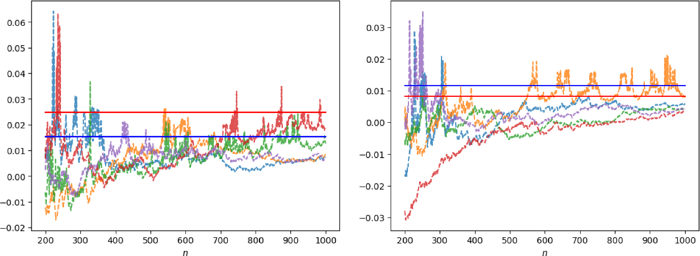
We then apply the standard moment method in random matrix theory[28, 29] along with the large N limit of \(t_=\textrm(\textrm(Z^n}^n))\) in our main theorem 4.1:

$$\begin t_=\frac(k+1)^\sqrt^+ O(\sqrt^) \end$$

(C.9)

to derive a rescaled semicircle law for the random matrix X in the probability measure \(Q_(X)[dX]\).

We introduce a rescaled variable:

$$\begin \tilde=\sqrt}X. \end$$

(C.10)

Let \(\tilde_\le \tilde_ \le \cdots \le \tilde_\) be the eigenvalues of the rescaled Hermitian matrix \(\tilde\). We define the spectral density of the eigenvalues \(\_, 1\le i \le N\}\) of \(\tilde\) on a real line \(\mathbb \):

$$\mu _(\tilde)=\frac\sum _^\delta (\tilde-\tilde_).$$

The resolvent \(\frac\textrm(\frac})\) of the random matrix \(\tilde\) is equal to the Stieltjes transformation \(S_}(w)\) of the density \(\mu _\):

$$S_}(w)=\int _}\frac}d\mu _(\tilde)=\frac\sum _^\frac_}=\frac\textrm\left( \frac}\right) .$$

We then compute the large N limit of the expectation value of the resolvent with respect to the probability measure \(Q_(X)[dX]\) defined earlier:

$$\begin&E_\left( \frac\textrm(\frac})\right) =\int [dX] \frac\textrm\left( \frac}X}\right) Q_(X)\\&=\int [dX]d\lambda d\lambda ^\widetilde\frac\textrm\left( \frac}\hat}\right) \left| X,\lambda \right\rangle \left\langle X,\lambda \right| \widetilde\\&=\widetilde\frac\textrm\left( \frac}\hat}\right) \widetilde. \end$$

Here, we denote expectation values with respect to the probability measure \(Q(X)_[dX]\) as \(E_(\cdots )\). Recalling \(\hat\!=\!\frac}(\hat+\hat)}\) and \(F(u,v)\!=\!\frac+v\hat})}=\sum _\left( m+n\\ m\end}\right) t_u^mv^n\), we apply the result \(t_=\frac(k+1)^\sqrt^+ O(\sqrt^)\). This yields:

$$\begin&\widetilde\frac\textrm\left( \frac}\hat}\right) \widetilde\\&\quad =\frac\widetildeF\left( \frac},\frac}\right) \widetilde\\&\quad =\frac \sum _^\left( 2n\\ n\end}\right) \widetildet_\widetilde(w\sqrt)^\\&\quad = \sum _^C_w^\\&\qquad +O(N^). \end$$

Here, \(\=\frac\left( 2n\\ n\end}\right) , n=0,1,\cdots \}\) are the Catalan numbers. From these calculations, we obtain the large N limit of the expectation value of \(S_}(w)\):

$$\begin \lim _E_(S_}(w))=\sum _^C_w^=\frac-4}} \quad w \in \mathbb ^=\| \textrm(z)>0\}. \end$$

Here, w is constrained to the upper half of the complex plane. The large N limit of the expectation value of the density \(\mu _(\tilde), \tilde\in \mathbb \) is obtained by the inverse Stieltjes transformation:

$$\begin \lim _ E_(\mu _(\tilde))=-\lim _}\textrm\(S_}(\tilde+i\epsilon ))\}=\frac\sqrt^2} \mathbb _(\tilde). \end$$

Here, \(\mathbb _(\tilde)\) is the characteristic function on the interval \([-2,2]\). This result is the renowned Wigner semicircle law. Converting back to the original matrix \(X=\sqrt}\tilde\), we obtain the following renormalized Wigner semicircle law:

Proposition C.1

Let \(Q_(X)[dX]\) be the probability measure on the space of \(N \times N\) Hermitian matrices as defined by (C.7). Let \(, 1\le i \le N}\) be the set of eigenvalues of X. The density of eigenvalues is given by \(\rho _(x)=\frac\sum _^\delta (x-x_)\). Then, in the large N limit, the leading term of the expectation value of \(\rho _(x)\) satisfies a renormalized (rescaled) semicircle distribution:

$$\begin E_(\rho _(x))=\frac\sqrt\mathbb _(x)+\text \quad \text \quad N \rightarrow \infty \end$$

(C.11)

where the radius is given by \(R=\frac\).

Physical interpretation: \(\frac\) is the filling factor of the quantum hall fluid

In the matrix model, the matrices \(\hat\) and \(\hat\) can be interpreted as non-commutative coordinates of electrons moving on a plane subjected to an external constant magnetic field B [1][3]. The harmonic potential \(Tr(\hat^2+\hat^2)\) confines the electrons within a disc centered around the origin of the plane. By diagonalizing the matrix \(X=UxU^\), where \(U \in U(N)/U(1)^\) and \(x=diag(x_1,x_,\cdots ,x_)\), the wave functions of the matrix model can be seen as functions of the variables U, \(x=diag(x_1,x_,\cdots ,x_)\), and \(\bar\):

$$\begin \Psi (x,U,\lambda )=\left\langle X=UxU^,\lambda \right| \left| phys\right\rangle \end$$

(C.12)

The wave function in (C.12) describes a quantum N-particle system in which each particle carries an internal U(p) spin in the representation \(\textrm^(\mathbb ^)\). The Hamiltonian of the matrix model is precisely that of a higher-spin extension of the Calogero model. For further mathematical details, we refer the reader to [7,8,9, 18].

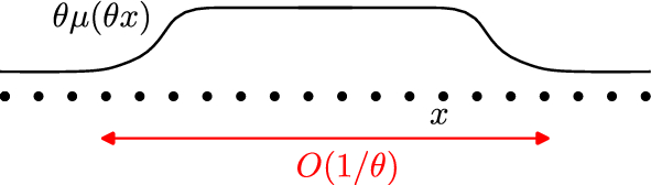
In the following, we focus first on the abelian case \(p=1\). The eigenvalues \((x_,x_,\cdots ,x_)\) are considered as the positions of the Calogero particles. In the context of the quantum Hall effect, the y coordinates of the particles correspond to the momenta of the eigenvalues \((x_,x_,\cdots ,x_)\). This implies that the y coordinates are spread out across the plane. The emergence of the semi-circle law distribution of the ground state wave function (C.11) can be understood as arising from a circle law distribution from the perspective of the quantum Hall fluid. The following pictureFootnote 8 illustrates our physical interpretation:

Let us compute the filling factor. From the rescaled semicircle law (C.11) distribution, the radius of the circle is \(R=\sqrt\). The area of the circle is \(Area=2\pi (k+1)N/B\). The number of magnetic flux that passes through the droplet is

$$\begin N_=Area \times \frac=(k+1)N. \end$$

(C.13)

Here, the charge of elecrons e and the planck constant \(\hbar \) are set to one. From these we obtain the filling factor as the ratio of the number of electrons and the number of magnetic flux that passes through the droplet:

$$\begin \nu =\frac}=\frac. \end$$

(C.14)

Let us calculate the filling factor. Using the rescaled semicircle law (C.11), we find that the radius of the circle is \( R = \sqrt} \). The area of the circle is \( \text = \frac \). The number of magnetic flux quanta passing through the droplet is given by:

$$\begin N_=Area \times \frac=(k+1)N. \end$$

Here, we have set the charge of electrons e and the Planck constant \(\hbar \) to one. With this information, we can compute the filling factor as the ratio of the number of electrons to the number of magnetic flux quanta passing through the droplet:

$$\begin \nu = \frac} = \frac. \end$$

(C.15)

Recall in in Sect. 4.2, we show that the central charge of the large N limit algebra \(\widehat(1)}_}\) is expressed as:

$$\begin c=\lim _(n+1)\tilde_=\frac. \end$$

Here, \(\tilde_=\sqrt^ t_ \). Additionally, recall that our derivation of the rescaled semicircle law (C.11) relies on the result \(\lim _(n+1)\tilde_=\frac\) . Therefore, we justify our claim that the central charge of the large N limit algebra is equal to the filling factor of the corresponding quantum Hall droplet.

This result is consistent with previous works on the matrix model concerning the quantum Hall effect [1, 3, 8], providing validation for the scaling factor chosen in this paper (See (4.18)(4.19)). Additionally, we note the work [20], where the authors also derived a semicircle law using saddle point approximation, while our derivation of this semicircle law relies on the moment method and the large N limit of the operators \(t_, n\ge 0\). The radius of the semicircle law (C.11) agrees with the one in [20].Footnote 9

The case \(p>1\): \(\frac\) is the filling factor of the quantum Hall fluid In the case \(p>1\), we consider a special situation: N is divided by p. Let \(N=pM\). In this situation (see 4.6), the ground state is unique (i.e., there is no degeneracy):

$$\begin \left| \textrm;N=pM\right\rangle =\prod _^[\epsilon ^i_\cdots i_}B(0)_\cdots i_}B(1)_\cdots i_}\cdots B(M-1)_\cdots i_}]^\left| 0\right\rangle \end$$

(C.16)

where

$$B(n)_i_\cdots i_}=\sum _,a_,\cdots a_ \le p} \epsilon _a_\cdots a_}(}^}}^n)_} (}^}}^n)_} \cdots (}^}}^n)_}$$

Let \(\widetilde;N=pM\right\rangle }\) be a normalized ground state:

$$\widetilde;N=pM\right| }\widetilde;N=pM\right\rangle }=1$$

Before we show the main proposition C.2, we need a lemma:

Lemma C.1

$$\begin t_\left| \textrm;N=pM\right\rangle =(k(M-1)+N)\textrm(Z^)\left| \textrm;N=pM\right\rangle . \end$$

(C.17)

Proof

Recall \(t_=\frac(\textrm(Z^ZZ^)+\textrm(Z^Z^Z)+\textrm(ZZ^Z^))\). When computing \(t_\left| \textrm;N=pM\right\rangle \), the element Z in \(t_\) will contract with:

1.

\(Z^\)’s in \(t_\). These contractions yield the term \(N\textrm(Z^)\left| \textrm;N=pM\right\rangle \) on the right-hand side of (C.17).

2.

\(Z^\)’s in \(\prod _^[\epsilon ^i_\cdots i_}B(0)_\cdots i_}B(1)_\cdots i_}\cdots B(M-1)_\cdots i_}]^\). Using the elementary fact that

$$\begin C(\,\)=\epsilon ^i_\cdots i_}(}^}}^})_}(}^}}^})_}\cdots (}^}}^})_}=0 \end$$

if there exist \(1<l_<l_<\cdots<l_<N\) such that \(n_}=n_}=\cdots =n_}\). It follows that the Wick contractions of Z in \(t_\) with \(Z^\)’s in \(B(0)_\cdots i_}B(1)_\cdots i_}\cdots B(M-2)_\cdots i_}\) will contribute zero. The Wick contractions of Z with \(Z^\)’s in \(B(M-1)_\cdots i_}\) give:

$$\begin&k(M-1)\i_\cdots i_}B(0)_\cdots i_}B(1)_\cdots i_}\cdots B(M-2)_\cdots i_}B(M)_\cdots i_}\cdot \\&\prod _^[\epsilon ^i_\cdots i_}B(0)_\cdots i_}B(1)_\cdots i_}\cdots B(M-1)_\cdots i_}]^\}\left| 0\right\rangle \\&=k(M-1)\textrm(Z^)\prod _^[\epsilon ^i_\cdots i_}B(0)_\cdots i_}B(1)_\cdots i_}\cdots B(M-1)_\cdots i_}]^\left| 0\right\rangle . \end$$

Here, we have used:

$$\begin&\epsilon ^i_\cdots i_}B(0)_\cdots i_}B(1)_\cdots i_}\cdots B(M-2)_\cdots i_}B(M)_\cdots i_}\\&=\textrm(Z^)\epsilon ^i_\cdots i_}B(0)_\cdots i_}B(1)_\cdots i_}\cdots B(M-1)_\cdots i_}, \end$$

which follows from a \(p>1\) generalization of relation (5.43) (as a corollary of (5.36)).

\(\square \)

The following proposition serves as evidence supporting Conjecture 4.1.

Proposition C.2

Assume in the limit: \(N=pM\), \(M \rightarrow \infty \), the operators \(\, n=0,1,2\cdots \}\) have leading order \(\sqrt^}\), i.e

Then we have:

$$\begin \widetilde;N=pM\right| }t_\widetilde;N=pM\right\rangle }=\frac\left( \frac\right) ^N^+O(N^) ,\quad N \rightarrow \infty . \end$$

(C.18)

Proof

Assume

then Proposition 3.2 implies that we have the following large N commutation relations

$$[t_,t_]=(n+2)t_+O(N^).$$

Let us denote

$$d(n):=\widetilde;N=pM\right| }t_\widetilde;N=pM\right\rangle }.$$

The ground state expectation value of C.18 is

$$\begin \widetilde;N=pM\right| }[t_,t_]\widetilde;N=pM\right\rangle }=(n+2)d(n+1)+O(N^). \end$$

(C.19)

It follows from Lemma C.1 that

$$\begin t_\widetilde;N=pM\right\rangle }=(k(M-1)+N)\textrm(Z^)\widetilde;N=pM\right\rangle }. \end$$

(C.20)

Taking the adjoint of the above and we get

$$\begin \widetilde;N=pM\right| }t_=(k(M-1)+N) \w