D-PINNS: distributional physics-informed neural networks

Consider a pharmacokinetic (PK) system described by a system of ODEs of the form:

$$\begin \begin \dfrac(t)} = \varvec(\varvec(t), t, \varvec), \quad \varvec(0) = \varvec_0 \end \end$$

(1)

where \(\varvec(t) \in \mathbb ^n\) denotes the vector of drug concentrations across \(N_c\) compartments, \(\varvec(\cdot )\) denotes the right-hand side of the ODE system, defining the system dynamics, \(\varvec_0\) specifies the initial condition, and \(\varvec\) represents the parameters of the ODE system. The solution to this system can be approximated by a neural network \(\widehat}(t)\), which takes time \(t \in [0, T]\) as input and produces estimated concentration values. Here, \(\varvec}}\) denotes the trainable parameters of the neural network, i.e., its weights and biases.

The key idea of PINNs is to incorporate knowledge of the system’s dynamics into the loss function through the residual of the ODE system, defined as:

$$\begin \begin \varvec}(t, \varvec) = \dfrac}(t)} - \varvec(\widehat}(t), t, \varvec) \end \end$$

(2)

where \(\frac\) denotes the time derivative of the neural network output. Although various numerical schemes are possible, PINNs typically use automatic differentiation to compute this derivative because it provides both accuracy and numerical stability [20]. The total loss function used to train the PINN is composed of three terms:

$$\begin \begin \mathcal _}= \lambda _} \mathcal _} + \lambda _} \mathcal _} + \lambda _} \mathcal _} \end \end$$

(3)

where \(\mathcal _}\), \(\mathcal _}\), and \(\mathcal _}\) are the ODE, initial condition and data loss terms, and \(\lambda _}\), \(\lambda _}\), and \(\lambda _}\) are the corresponding loss weights. The individual loss terms are defined as:

$$\begin \begin \mathcal _} = \dfrac|} \sum _^} \left\| \left. \dfrac}(t_j)} \right| _} - \varvec(\widehat}(t_j), t_j, \varvec) \right\| _2^2 \end \end$$

(4)

$$\begin \begin \mathcal _}= \dfrac \left\| \widehat}(0) - \varvec_0 \right\| _2^2 \end \end$$

(5)

$$\begin \begin \mathcal _}= \dfrac}|} \sum _^}} \left\| \widehat}(t_j) - \varvec(t_j) \right\| _2^2 \end \end$$

(6)

where \(N_\) denotes the collocation points at which the residuals are evaluated, \(N_c\) reprents the number of compartments, \(N_}\) corresponds to the number of observations, and \(\left. \frac\right| _}\) indicates that the derivative is computed via automatic differentiation of the neural network. The training process involves jointly optimising the neural network parameters \(\varvec_}\) and the ODE system parameters \(\varvec\) by minimising a composite loss function that integrates both the system dynamics and the observed data.

The core principle of D-PINNs lies in incorporating both the mean and variance of the system’s state into the optimisation process by adopting appropriate distributional assumptions. In this framework, the neural network does not predict concentration values directly, but instead outputs the mean and variance of the concentration, which serve as statistical summaries of the observed data. Consequently, each concentration value, previously modelled as a single deterministic output, is now represented by two outputs: one for the predicted mean and one for the predicted variance. These predictions are used inside a sampling framework that employs the ODE system to compute the ODE loss term. Figure 2 presents a simplified schematic of the D-PINN framework, offering a high-level view of its key components prior to the detailed formulation.

Fig. 2

Schematic representation of the D-PINN algorithm applied to a simple one-dimensional problem. This schematic highlights the core component of the algorithm: the computation of the ODE loss term. The method integrates a neural network (NN) with a system of ordinary differential equations (ODEs). At its core, the NN outputs the estimated mean and variance of the concentration over time, which are used to generate noisy concentration samples. These samples are then denoised and passed through the ODE system to compute the time derivatives of the mean and variance. These are directly compared to the corresponding derivatives from automatic differentiation of the neural network to calculate the ODE loss

Building on the schematic representation, we now present the full mathematical formulation of the D-PINN framework. This extension of the original PINN formulation introduces a total loss function that simultaneously accounts for the mean and variance of the predicted system state:

$$\begin \begin \mathcal _} &= \lambda _}^} \mathcal _}^} + \lambda _}^} \mathcal _}^} + \lambda _}^} \mathcal _}^} \\&\quad+ \lambda _}^} \mathcal _}^} + \lambda _}^} \mathcal _}^} + \lambda _}^} \mathcal _}^} \end \end$$

(7)

with:

$$\begin \begin \mathcal _}^}= \dfrac|} \sum _^} \left\| \left. \dfrac[\varvec(t_j)]}} \right| _} - \left. \dfrac[\varvec(t_j)]} \right| _} \right\| _2^2 \end \end$$

(8)

$$\begin \begin \mathcal _}^} = \dfrac|} \sum _^} \left\| \left. \dfrac[\varvec(t_j)]}} \right| _} - \left. \dfrac[\varvec(t_j)]}} \right| _} \right\| _2^2 \end \end$$

(9)

$$\begin \begin \mathcal _}^} = \dfrac \left\| \widehat[\varvec(t_0)]} - \mathbb [\varvec_(\varvec)] \right\| _2^2 \end \end$$

(10)

$$\begin \begin \mathcal _}^}= \dfrac \left\| \widehat[\varvec(t_0)]} - \textrm[\varvec_0(\varvec)] \right\| _2^2 \end \end$$

(11)

$$\begin \begin \mathcal _}^} = \dfrac}|} \sum _^}} \left\| \widehat[\varvec(t_j)]} - \mathbb [\varvec(t_j)] \right\| _2^2 \end \end$$

(12)

$$\begin \begin \mathcal _}^} = \dfrac}|} \sum _^}} \left\| \widehat[\varvec(t_j)]} - \textrm[\varvec(t_j)] \right\| _2^2 \end \end$$

(13)

where \(\widehat[\varvec(t_j)]}\) and \(\widehat[\varvec(t_j)]}\) denote the mean and variance of the concentration at time point \(t_j\) predicted by the NN, while \(\mathbb [\varvec(t_j)]\) and \(\textrm[\varvec(t_j)]\) correspond to the observed mean and variance of the concentration at time point \(t_j\). The notation \(\left. \frac\right| _}\) indicates that the derivative is estimated directly through the ODE system using sampling.

We assume a single homogeneous population from which individual-specific parameters are drawn. In this setting, the population-level variability corresponds directly to interindividual variability, reflecting variability among individual subjects around a single common population mean. The aim of D-PINNs is to estimate the population distribution of the ODE parameters \(\varvec\), described by distributional parameters \(\varvec_\), based on estimates of the concentration mean and variance. The model accounts for interindividual variability explicitly through the distribution of \(\varvec\). Residual variability is assumed to originate solely from measurement error, including sources such as assay variability and sample handling error. As a result, the observed concentrations reflect both interindividual variability and measurement error. Accordingly, the associated sample means and variances are noisy estimates of the true underlying moments. Assuming a log-normal error model, the noise-free concentration at each time point, denoted by \(\varvec^}(t)\), can be related to the observed concentration \(\varvec(t)\) via:

$$\begin \varvec(t)&= \varvec^}(t) \cdot e^ , \quad \varvec \sim \mathcal (0, \sigma ^2) \end$$

(14)

where \(\varvec\) is the residual error on the log scale, representing measurement error, and \(\sigma\) is the residual standard deviation on the log scale. Parameter \(\sigma\) is treated as a trainable parameter in this framework. The distinction between \(\varvec^}(t)\) and \(\varvec(t)\) is critical, as it allows the model to account for residual variability and disentangle noisy observations from the underlying true concentrations that are used in the ODE system, as will be elaborated later in this section.

At each iteration, a forward pass with the current estimate of \(\varvec_}\) yields updated predictions for the noisy concentration mean and variance, \(\widehat[\varvec(t)]}\) and \(\widehat[\varvec(t)]}\), respectively. These predictions, along with the updated distributional parameter estimates \(\varvec_\), are appropriately transformed to parameterise a predefined joint distribution, \(p( \varvec(t), \varvec)\), from which samples of \(\varvec(t)\) and \(\varvec\) are drawn. Residual errors are sampled using the current estimate of the residual standard deviation \(\sigma\) and are applied to Eq. 14 to correct for measurement noise. This denoising step yields sampled estimates of the true concentration, \(\varvec^}(t)\). For each sampled instance (i), the corresponding denoised concentration \(\varvec^, (i)}(t)\) and parameter vector \(\varvec^\) are subsequently used to compute the respective time derivative:

$$\begin \begin \dfrac^,(i)}(t)} = \varvec(\varvec^, (i)}(t), t, \varvec^) \end \end$$

(15)

The resulting distribution of derivatives is then used to compute the ODE-based estimates of the time derivatives of the denoised concentration mean and variance, as follows:

$$\begin \begin \left. \dfrac[\varvec^}(t)]} \right| _}&= \dfrac}|} \sum _^}} \dfrac^,(i)}(t)} \end \end$$

(16)

$$\begin \begin \left. \dfrac[\varvec}}(t)]} \right| _}&= \dfrac}| - 1} \sum _^}} \Bigg [ \left( C^, (i)}(t) - \mathbb [\varvec^}(t)] \right) \cdot \\&\quad \hspace\left( \dfrac^,(i)}(t)} - \left. \dfrac[\varvec^}(t)]} \right| _} \right) \Bigg ] \end \end$$

(17)

where \(N_}\) represents the total number of drawn samples. A full derivation of these expressions, along with the associated assumptions, is provided in Appendix A. The final step consists of reconstructing the ODE-based derivatives of the observed concentration mean and variance from the denoised estimates via the following transformation:

$$\begin \left. \frac[C(t)]}\right| _}&= e^/2} \cdot \left. \frac[C^}(t)]} \right| _} \end$$

(18)

$$\begin \left. \frac[C(t)]} \right| _}&= e^ \cdot \left[ 2 \cdot \mathbb [C^}(t)] \cdot \left. \frac[C^}(t)]} \right| _} \cdot \left( e^ - 1 \right) \right. \nonumber \\&\quad \left. + e^ \cdot \left. \frac[C^}(t)]} \right| _} \right] \end$$

(19)

The derivation of Eqs. 18 and 19 is provided in Appendix B. This parameterisation allows the model to simultaneously estimate both the population-level distribution of the ODE parameters and the measurement error in the observed concentrations. The ODE-based estimates of the observed mean and variance derivatives are then compared against those obtained via automatic differentiation of the NN, through Eqs. 8 and 9, to compute the ODE-related loss terms. When the system’s initial conditions depend on the ODE parameters \(\varvec\), the same sampling workflow is applied to estimate \(\mathbb [\varvec_0(\varvec)]\) and \(\textrm[\varvec_0(\varvec)]\). The trainable parameters of the system, namely the neural network parameters \(\varvec_}\), the distributional parameters \(\varvec_\), and the residual standard deviation \(\sigma\), collectively denoted by \(\varvec\), are optimised by minimising the total loss function. Algorithm 1 outlines the computational workflow of the D-PINNs framework, while Fig. 2 illustrates its core components in the context of a simple one-compartment ODE system.

Algorithm 1Case study 1: simulated data from a one-compartment pharmacokinetic model

The aim of case study 1 is to illustrate the application of D-PINNs for estimating population-level pharmacokinetic parameters. To showcase the capabilities of the methodology, we selected a simple one-compartment model with intravenous (IV) bolus dosing as a representative system. This model was chosen for its simplicity, widespread use in early-phase pharmacokinetic studies, and its suitability as a tractable framework for evaluating new inference approaches. Simulated data were generated using predefined population-level pharmacokinetic parameters. The performance of the D-PINN framework was then assessed by comparing the estimated parameters to the reference values used during simulation. The modelling workflow of case study 1 is illustrated in Fig. 3.

Fig. 3

Modelling workflow for Case Study 1. A predefined population parameter distribution is used to generate a virtual cohort and simulate IV concentration–time profiles. After adding measurement noise and sampling at predefined time points, the concentration mean and variance are computed. These summary statistics are then provided as training data to the D-PINN model, which estimates the mean and variance of each population parameter. The estimated distributions are finally compared to the ground-truth distributions used to generate the virtual cohort

Pharmacokinetic system

The one-compartment pharmacokinetic model describes a simplified system in which the drug is assumed to distribute instantaneously and uniformly within a central compartment. Following a bolus IV injection, the drug enters directly into the central compartment. The model is schematically presented in Fig. 4.

Fig. 4

Schematic presentation of the simple, one-compartment pharmacokinetic model

The ODE system that expresses the pharmacokinetic model is presented in Eqs. 20 - 21. It consists of a single state describing the concentration evolution of the drug in plasma over time, C(t). The pharmacokinetics of the system are characterized by two parameters: the volume of distribution (\(V_d\)), which governs how extensively the drug partitions between plasma and peripheral tissues, and the elimination rate constant (\(k_e\)), which governs the rate at which the drug is removed from the system. At time zero, the initial concentration of the drug was set to the total dose divided by \(V_d\).

$$\begin \dfrac&= - k_ C(t) \end$$

(20)

$$\begin C(t_0)&= \frac} \end$$

(21)

Simulated data

The presented one-compartment model was used to simulate a cohort of 30 virtual patients, each characterized by individual pharmacokinetic parameters. These parameters were sampled from a multivariate population distribution and served as inputs to the ODE system to generate patient-specific plasma concentration-time profiles. Specifically, \(V_d\) and \(k_e\) were jointly sampled from a multivariate log-normal distribution. The population mean for \(V_d\) was set to \(15 \, \text \), with a coefficient of variation (CV) of \(10\%\). The mean of \(k_e\) was defined by specifying a mean half-life in blood equal to \(6 \, \text \) (\(k_e \approx 0.12\)), and its standard deviation was defined through a CV of \(40\%\). The correlation between \(V_d\) and \(k_e\) was varied to explore its impact on the inference process.

In the simulated scenario, a \(300 \, \text \) bolus intravenous dose was assumed, and plasma concentrations were computed at 0.5, 1, 2, 6, 12, and 24 h post-administration, reflecting a clinically relevant sampling schedule. To account for residual variability, a log-normal error model was used, with log-scale standard deviation set to \(\sigma = 0.1\). Thus, for each virtual patient k and observation time point \(t_j\), the observed concentration was generated using the following model:

$$\begin \log \varvec_k&= [\log V_, \log k_] \sim \textrm(\varvec, \Omega ) \end$$

(22)

$$\begin C_(t_j)&= C^}_(t_j) \cdot e^}, \quad \epsilon _ \sim \mathcal (0, \sigma ^2) \end$$

(23)

where \(\textrm\) denotes the multivariate normal distribution, \(\varvec\) and \(\Omega\) represent the mean vector and covariance matrix, and \(\epsilon _\) denotes the corresponding measurement error. The distributional parameters are thus defined as \(\varvec_ = [\varvec, \Omega ]\). The resulting data were summarized by computing the mean and variance at each time point and subsequently used as input for the D-PINN analysis. Therefore, the reported summary statistics at each time point reflect both interindividual pharmacokinetic variability and measurement noise.

D-PINN implementation

The objective of the case study is to demonstrate that, under the true structural and statistical models, D-PINNs can recover the pharmacokinetic parameter distribution using only aggregated plasma concentration data. Accordingly, the same ODE system was employed, and the D-PINN was configured to assume the same probability distribution for the system parameters as the one used during data simulation. At each iteration, the mean and variance estimates of the NN at time points \(t_j \in \ \cup T_\), \(\widehat[\varvec(t)]}\) and \(\widehat[\varvec(t_j)]}\), were used alongside the distributional parameters \(\varvec}\) to parameterise a joint probability distribution. Specifically, for each time point \(t_j\), \(j = 1, \cdots , N_\), and sample index \(i = 1, 2, \dots , N_}\), draws from the joint distribution over plasma concentration and ODE parameters were obtained as follows:

$$\begin \log C^(t_j), \log V_^, \log k_^ \sim \textrm(\varvec\varvec_}, \Omega _j') \end$$

(24)

where \(\varvec', \Omega _j'\) were constructed by first transforming \(\widehat[\varvec(t_j)]}\) and \(\widehat[\varvec(t_j)]}\) into their corresponding log-scale parameters by applying standard transformations from linear-scale moments to log-scale parameters of the log-normal distribution. The transformed estimates were then combined with the already log-transformed distributional parameters \(\varvec_\) to form \(\varvec'\) and \(\Omega _j'\) . While the mean and variance estimates are time-dependent, distributional parameters \(\varvec_\) remain fixed across time. Nevertheless, samples of \(V_d\) and \(k_e\) were drawn across time to better capture the range of parameters capable of reproducing the observed plasma statistical summaries. Additionally, to enable joint sampling of the ODE parameters and plasma concentration, the covariance matrix \(\Omega _j'\) also included the correlations between plasma concentration and ODE parameters. These correlation terms were assumed time-invariant and were treated as trainable parameters. Finally, sampled noisy concentrations were denoised using Eq. 14, and then mean and variance ODE-based time derivatives were computed by applying Eqs. 16 - 19.

In addition to the ODE-based loss, samples of \(V_d\) were also used to compute the initial condition loss terms. The neural network outputs the mean and variance of the observed concentrations, which reflect both biological variability and measurement noise. This should not be confused with the typical ODE initial conditions, which account only for biological variability. Consequently, the initial condition of the network must incorporate the effects of measurement noise. Specifically, samples of \(V_d\) at time \(t_0\) were used to estimate the observed initial concentration as:

$$\begin C^(t_0) = \frac}} \cdot e^ , \quad \epsilon \sim \mathcal (0, \sigma ^2) \end$$

(25)

These samples were then summarised to compute the mean and variance of the initial observed concentration. The resulting statistical summaries were incorporated into Eqs. 10 and 11, along with NN estimates \(\widehat[C](t_0)}\) and \(\widehat[C(t_0)]}\), to derive the initial condition loss.

Regarding implementation details, a simple feedforward NN was employed, consisting of two hidden layers with three nodes each. The tanh activation function was applied to all layers, while the output layer included the softplus transformation to ensure non-negative NN outputs. NN weights were initialised using the Glorot normal initialiser, and no loss regularisation was applied. The model was trained using the Adam optimizer with a learning rate of 0.0005. To further enhance model stability, gradient clipping was performed to constrain the Euclidean norm of all gradients to be less than 10. The impact of the number of samples \(N_}\), the number of collocation points \(N_\) and the choice of loss weights on predictive performance was assessed using simulations. All trainable parameters representing elements of the correlation matrix parameters were transformed using the tanh function to constrain their values within the [-1,1] interval. Similarly, all trainable parameters representing standard deviations were transformed using the softplus function with a small positive bias, to ensure strictly positive values.

Finally, the accuracy of each individual distributional parameter estimate \(\theta _^}\) was compared to the true parameter \(\theta _^\) using the absolute percentage error (APE), as defined in Eq. 26. The overall estimation accuracy across all \(N_}\) distributional parameters was evaluated using the mean absolute percentage error (MAPE), shown in Eq. 27.

$$\begin \textrm_p&=100\%\times \left| \frac^-\theta _^}^}\right| , \quad p=1,\dots ,N_} \end$$

(26)

$$\begin \textrm&=\frac}}\sum _^}\textrm_p \end$$

(27)

Case study 2: parameter estimation for a minimal physiologically-based pharmacokinetic model

The main goal of case study 2 is to employ D-PINNs in a real-world pharmacokinetic modeling estimation problem. For this purpose, a minimal physiologically based pharmacokinetic (mPBPK) model was implemented to simulate the kinetics of TAB008 (later marketed as Pusintin), a biosimilar monoclonal antibody (mAb) of bevacizumab (Avastin). The aggregated mAb plasma concentrations were also modelled using a Bayesian analogue implemented using the Markov chain Monte Carlo (MCMC) methodology to benchmark the speed and estimation performance of D-PINNs .

Monoclonal antibody data

The aggregated concentration data were drawn from a phase I clinical study of TAB008 [21]. The pharmacokinetic study included 49 healthy Chinese male subjects aged 18-45 years old, with body-weights ranging from 50 to 75 kg. Each subject received a single IV dose of 1 mg/kg of TAB008, administered over a 90-minute infusion. A sample was collected at 0.75 hours after the start of infusion, followed by five additional samples between 0 and 8 hours post-infusion. Sampling was further extended up to 99 days post administration to study long term kinetics. The online software PlotDigitizer [22] was used to extract the reported mean and standard deviation of serum concentrations over time from the published figure. In total, 15 measurements of aggregated plasma concentrations over time were extracted from the figure and used to estimate the pharmacokinetic parameters of the mAb.

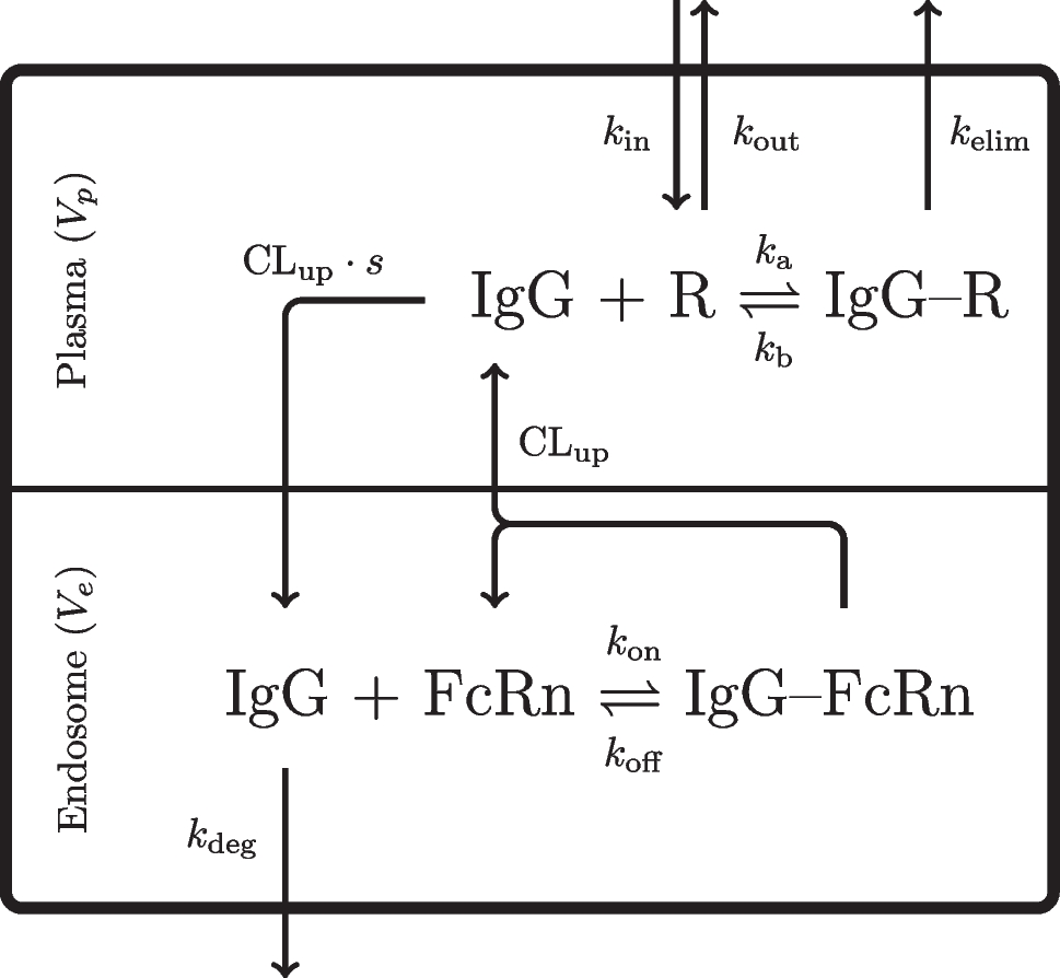
Minimal physiologically-based pharmacokinetic model

The implemented model follows a minimal modelling approach specifically designed to characterise mAb kinetics [23]. It assumes that convection is the primary mechanism driving mAb distribution into the extravascular space. Because mAbs exhibit limited permeability across cellular membranes, the interstitial fluid (ISF) compartment is considered the main extravascular space for distribution. Accordingly, tissues are grouped into two categories based on capillary structure: continuous or discontinuous. The discontinuous (leaky) group includes tissues such as the liver, kidney, and heart, whereas the continuous (tight) group includes muscle, skin, and adipose tissue. Transport of mAbs from plasma to ISF is governed by tissue-specific reflection coefficients, and lymphatic return to plasma is similarly regulated by a distinct reflection coefficient. A structural representation of the mPBPK model is shown in Fig. 5.

Fig. 5

Structural representation of the mPBPK model, redrawn and adapted from [23]. The current implementation considers that mAbs are eliminated only through the plasma compartment

The differential equations that describe the dynamics of the system follow the formulation of Cao et al. [23] and are provided below:

$$\begin&\frac} = \left[ \frac} +C_ \cdot L - C_ \cdot L_1 \cdot (1 - \sigma _1) \right. \nonumber \\&\qquad \qquad \left. - C_ \cdot L_2 \cdot (1 - \sigma _2) - C_\cdot CL_p\right] /V_ \end$$

(28)

$$\begin\frac} &= \left[ L_1 \cdot (1 - \sigma _1) \cdot C_ \right.\\&\left.\quad- L_1 \cdot (1 - \sigma _L) \cdot C_\right] /V_ \end$$

(29)

$$\begin\frac} &= \left[ L_2 \cdot (1 - \sigma _2) \cdot C_ \right.\\&\quad\left.- L_2 \cdot (1 - \sigma _L) \cdot C_\right] /V_ \end$$

(30)

$$\begin\frac}&= \Bigg[ L_1 \cdot (1 - \sigma _L) \cdot C_ + L_2 \cdot (1 - \sigma _L) \\& \cdot C_ - C_\cdot L \Bigg] /V_ \end$$

(31)

In Eqs. 28 to 31, \(C_\) denotes the plasma concentration, \(C_\) is the lymph concentration, and \(C_\) and \(C_\) are the concentrations in the tight and leaky and compartments, respectively. The term \(T_\) represents the IV infusion time, \(V_\) and \(V_\) denote the plasma and lymph volumes, and \(V_\) and \(V_\) correspond to the total ISF volumes in tight and leaky tissues. Moreover, L represents the total lymph flow, while \(L_1\) and \(L_2\) represent the lymph flow to tight and leaky compartments. Finally, \(CL_p\) denotes the clearance rate from plasma, \(\sigma _L\) is the lymphatic capillary reflection, and \(\sigma _1\) and \(\sigma _2\) represent the vascular reflection coefficients for the tight and leaky compartments, respectively. A detailed parameterisation of the model is provided in Appendix C.

The model imposes several physical constraints on the parameters. Specifically, both \(\sigma _1\) and \(\sigma _2\) must be lower than 1, since the extravasation rate cannot be higher than the total lymph flow (L). In addition, they must satisfy the inequality \(\sigma _1> \sigma _2\), since tight vascular endothelium tissues have a higher reflection than leaky tissues.

D-PINN implementation

The aggregated plasma concentration data were used to estimate plasma clearance, \(CL_p\), and the reflection coefficients of tight and leaky tissues, \(\sigma _1\) and \(\sigma _2\), respectively. Among these parameters, only \(CL_p\) was treated as a stochastic parameter to account for interindividual variability within the studied population. In contrast, point estimates were used for the reflection coefficients. This choice is supported by the physiological nature of the reflection coefficients, which characterise permeability through the capillary membranes, and are not expected to exhibit high interindividual variability. Apart from interindividual variability in clearance, the D-PINN implementation also incorporated variability in physiological parameters by sampling the body weight of virtual subjects from a uniform distribution defined by the minimum and maximum values (50 and 75 kg) reported in [21]. All physiological parameters dependent on body weight (\(V_, V_, V_, V_, L\), \(L_1\) and \(L_2\)) were adjusted accordingly (see Eqs. 65 to 72 in Appendix C). Finally, the administered dose was scaled based on the sampled body weight, according to the 1 mg/kg dosing regimen followed in the trial [21].

The output layer of the NN was adjusted to the availability of aggregated concentration data. Specifically, two nodes were used for the aggregated plasma concentration, representing the central tendency and spread of the plasma concentration, and a single output node was employed for each unobserved state, including the concentration in the lymph, tight and leaky tissues. The observed variance in the clinical data spanned a wide range (0.01–9), covering almost three orders of magnitude. To better scale this wide range and avoid the optimisation issues associated with large output disparities, we modelled the standard deviation instead of the variance. Data loss terms were linked only to the first two output nodes, while all initial condition loss terms were set to zero. The ODE-based derivative of the ODE loss term for the standard deviation was estimated using the following equation:

$$\begin \left. \frac[C(t)]} \right| _}&= \frac[C(t)]} \right| _}}[C(t)]}} \end$$

(32)

where \(\widehat[\varvec(t)]}\) is the standard deviation predicted by the NN and \(\left. \frac[C(t)]} \right| _}\) is computed using Eq. 19. To further facilitate NN convergence, we applied output scaling, a standard technique in NN training. Specifically, Min–Max scaling was applied to rescale the observed outputs to the 0–1 interval. The observed mean and standard deviation of the plasma concentration were transformed as follows:

$$\begin X_ = \frac -X_} - X_} \end$$

(33)

where \(X_\) and \(X_\) correspond to the minimum and maximum values observed for the mean and standard deviation of the plasma concentration. Since no data were available for the lymph, leaky and tight tissue concentrations, their outputs were scaled using the minimum and maximum values of the mean plasma concentration. To obtain the true parameter values and use them in the right-hand side of the ODE system, the NN outputs were subsequently mapped back to the original scale using the inverse transformation:

$$\begin X_ = X_\cdot (X_ - X_) + X_ \end$$

(34)

Finally, because AD produces derivatives of the scaled variables while the ODE system is expressed in unscaled variables, these derivatives were mapped back to the original scale before computing the ODE loss term, using the following transformation:

$$\begin \left. \frac[C(t)]_}}\right| _}= \left. \frac[C(t)]_}} \right| _} \\\cdot \left( \max \mathbb [C(t)] - \min \mathbb [C(t)] \right) \end$$

(35)

$$\begin \left. \frac[C(t)]_}} \right| _}= \left. \frac[C(t)]_}} \right| _} \\ \cdot \left( \max \textrm[C(t)] - \min \textrm[C(t)] \right) ^ \end$$

(36)

The unscaled standard deviation was internally converted to variance, and Algorithm 1 was followed. Similar to case study 1, at each iteration, the predictions of the NN along with the distributional parameters of \(CL_p\) were used to construct the joint probability distribution. At each time point \(t_j\), samples were drawn from the joint distribution over the plasma concentration and the \(CL_p\) parameter, as described in Eq. 37.

$$\begin \log C^_(t_j), \log CL_}^&\sim \textrm(\varvec\varvec_}, \Omega _j') \end$$

(37)

where \(\varvec\) and \(\Omega _j'\) were constructed using log transformations similar to the ones described in the first case study. The reflection coefficients were parameterised to respect their physical constraints. Specifically, \(\sigma _1\) was mapped to the interval (0, 1) using an inverse-logit transformation of an unconstrained auxiliary variable \(\sigma _\), while \(\sigma _2\) was defined as the product of \(\sigma _1\) and the inverse-logit transformation of unconstrained auxiliary variable \(\sigma _\). This ensured that both coefficients remained below 1 and that \(\sigma _1 \ge \sigma _2\) at all times. Finally, a log-normal error model was applied to account for measurement error and derive the noise-free concentrations (Eq. 14).

The NN architecture was kept simple, consisting of two hidden layers with 30 neurons each, using the tanh() activation function. After a tuning procedure, the number of collocation points was set to 100, which ensured a dense grid over the time span of the simulation while keeping computational cost low. The number of virtual subjects was also set to 100. NN weights were initialised using the Glorot normal initialiser, and no loss regularisation was applied. The model was trained with the ADAM optimizer for 70000 iterations, with an initial learning rate of 5e-04 and an exponential decay schedule that reduced the learning rate by 1% every 1000 iterations. All loss terms contributed equally to the total loss by assigning a unit weight to each term.

Benchmarking with Markov Chain Monte Carlo (MCMC)

The strengths and weaknesses of a methodology can be assessed through comparison with alternative approaches. Towards this direction, case study 2 was also modelled using a Markov-chain Monte Carlo analogue introduced in [19]. Stan [24], which provides an efficient implementation of the NUTS algorithm [25], was used for modelling. The summarised concentration data were reanalysed under this framework. The same number of virtual subjects as in the D-PINN model was considered (\(N_=100\)), with each subject receiving a pre-assigned body weight sampled from a uniform distribution that was kept fixed for the entire simulation. At every iteration, individual clearance parameters and the two reflection coefficients were sampled and applied to solve the ODE system for each subject. At the study sampling times, measurement error was added, the simulated concentrations were aggregated using the mean and standard deviation and were finally compared against the reported summary statistics.

A three-tiered hierarchical model was employed to characterise the data. The first tier defined a likelihood on the summary statistics of the plasma concentrations, assuming log-normal observational errors for both the mean and the standard deviation. The second tier described the individual-level parameters, and the third tier covered the population level, assigning prior distributions to the population parameters. For the reflection coefficients, sampling was performed at the population level, whereas for clearance, a population mean and interindividual variability were used to sample individual clearance values.The statistical formulation is presented in Eqs. 38–46.

First stage

$$\begin \log \!\big (\mathbb [C(t_i)]\big )&\sim N\!\left( \log \!\big (\widehat[C(t_i)]}\big ), \; \sigma _}^2 \right) \end$$

(38)

$$\begin \log \!\big (\textrm[C(t_i)]\big )&\sim N\!\left( \log \!\big (\widehat[C(t_i)]}\big ), \; \sigma _}^2 \right) \end$$

(39)

Second stage

For each subject j, clearance follows a lognormal distribution:

$$\begin \begin CL_j&= e^} + \tau _}\, z_j}, \quad z_j \sim N(0,1), \end \end$$

(40)

The PBPK model produces individual predictions, \(\hat_k(t_i)\), and then measurement error is added:

$$\begin C_k(t_i)&= \hat_k(t_i)\cdot e^}, \quad \epsilon _ \sim N(0,\sigma ^2) \end$$

(41)

The predicted mean across subjects is computed as:

$$\begin \widehat[C(t_i)]}&= \frac}} \sum _^}} C_k(t_i). \end$$

(42)

The predicted standard deviation across subjects is:

$$\begin \widehat[C(t_i)]}&= \sqrt} - 1} \sum _^}} \left( C_k(t_i) - \widehat[C(t_i)]} \right) ^ }. \end$$

(43)

The reflection coefficients were transformed similar to the D-PINN model as:

$$\begin \sigma _1&= \textrm^(\sigma _}), \end$$

(44)

$$\begin \sigma _2&= \sigma _1 \cdot \textrm^(\sigma _}). \end$$

(45)

Third stage

$$\begin \begin \mu _}&\sim N\!\left( \mu _}^,\; \sigma _}}^\right) \\ \tau _}&\sim N_\!\left( \tau _}^,\; \sigma _}}^\right) \\ \sigma _}&\sim N_(0,1) \\ \sigma _}&\sim N_(0,1) \\ \sigma _}&\sim N(0,1) \\ \sigma _}&\sim N(0,1) \end \end$$

(46)

where \(N_\) is the half normal distribution. The transformed hyperparameters \(\mu _}^, \sigma _}}^\) and \(\tau _}^, \sigma _}}^\) are computed in the transformed data block to map priors specified on the normal scale to the log scale.

Software and code availability

All models were run on a computer with an Intel Core i7-8700 (3.2 GHz), 16 GB RAM and windows 10 OS. All computations relevant to D-PINNs were facilitated using the python package DeepXDE (v.1.9.3) [26], and in particular the Tensorflow (v.2.1.3) interface [