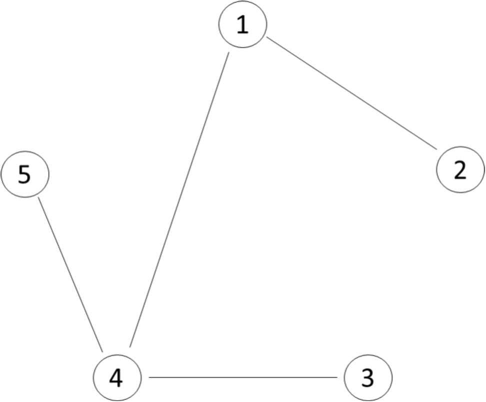
In order to capture the spatial and the temporal properties of columnar neurons in the fly visual system, I simulated the neural activity in five adjacent columns arranged in a linear way (Fig. 2A). Each column contained 65 cell types, each with identical properties across all columns. The connectivity within each column (Fig. 2B) was set according to connectomic data (Shinomiya et al., 2019) with the strength of each connection corresponding to the number of synapses and the sign based on the known transmitter phenotype of each cell and its postsynaptic receptor. The connectivity between neighboring columns (Fig. 2C) was constructed in the same way, except for L4 cells, whose branches in neighboring columns were assumed to be electrically isolated. This resulted in a network of 325 neurons with an overall connectivity combining the intra- and inter-columnar connections (Fig. 2D). While such a linear arrangement of only five columns might seem limited and somewhat unnatural, given the 2-dimensional, hexagonal arrangement of about 800 optical columns in the fly, it suffices for the purpose of the current study which investigates the temporal dynamics of the individual elements based on the connectivity between the neurons within each column and the ones between neurons in immediate neighboring ones.

Layout of network model. (A) Schematic of the circuit. Five adjacent columns, arranged in a linear way, were simulated. (B) Intra-columnar connectivity matrix containing the synaptic weights between all 65 columnar elements. (C) Same as B, but for inter-columnar connectivity. (D) Resulting overall connectivity matrix for all 325 network elements. Data from (Shinomiya et al., 2019) split into intra- and inter-columnar connectivity by Janna Lappalainen

I modeled each neuron as a single-compartment, conductance-based, graded-potential element (for details, see Methods). Each neuron received excitatory and inhibitory input according to the overall connectivity matrix. Importantly, each neuron type was given two free parameters, an input and an output gain. By applying the input gain of a neuron to all its presynaptic input neurons and the output gain uniformly to all its postsynaptic downstream neurons, the relative strength of connectivity as set by the connectivity matrix was preserved. All neurons were given the same capacitance and leak conductance, and, thus, had uniform intrinsic passive membrane properties. Lamina cells L1-3 are the first neurons postsynaptic to photoreceptors R1-6, and, therefore, should be important for shaping the response properties of downstream medulla neurons. L1 and L2 are known to respond to a light pulse by a transient hyperpolarization with a typical ‘sag’ in the neuron’s membrane potential, followed by a rebound excitation after the light has been turned off (Zettler & Straka, 1987; Laughlin et al., 1987). Such a response can be caused by two different mechanisms: (1) Low-pass filtering the light response with two different time-constants and taking the difference between the two outputs (Fig. 3A, B) or by (2) intrinsic, active membrane properties of the lamina cells (Fig. 3C-F). In the latter case, the current leading to the response sag could be a depolarizing current activated by hyperpolarization such as the H-current (Fig. 3C, D), or the deactivation of a hyperpolarizing current, such as a non-inactivating K-current (Fig. 3E, F). Transcriptomic data indicated a high expression level of the gene coding for an HCN-channel (FlyBase ID: FBgn0263397), responsible for an H-current, in lamina cells L1, L2 and L5 (Davis et al., 2020). I, therefore, incorporated such a current in lamina cells in some of the simulations. With each neuron type having an input and an output gain, the total number of free parameters in the model amounted to 130. If the model incorporated an H-current, 5 additional parameters were used to describe the maximum conductances in the five lamina cells and 3 parameters to characterize the voltage-dependence of the H-current activation curve and time-constant (for details, see Methods).

Different ways to produce transient responses. (A) Responses of a 1 st (in red) and of a 2nd order lowpass filter (in blue) to a pulse of 1 s duration. (B) The unbalanced difference of 1 st and 2nd order signals leads to a transient hyperpolarization response. (C) Activation characteristic (in blue) and voltage-dependent time-constant (in orange) of a H-current. (D) Response of a model neuron with an H-current to a hyperpolarizing current injection. (E) Activation characteristic (in blue) and time-constant (in orange) of a non-inactivating K-current. (F) Response of a model neuron with a K-current to a hyperpolarizing current injection

I modeled a linear array of five adjacent columns and injected a depolarizing current step in photoreceptors R1 to R8 within the central column, equivalent to a light pulse delivered locally. Its spread into the other neighboring columns was used to determine the spatial receptive field of each neuron type in the central column (for details, see Methods). To account for the fact that experimental data were derived from calcium imaging, the voltage responses of the model neurons were finally fed through a 1 st -order low-pass filter with 50 ms time-constant. To fit the model responses to the data, an overall error or cost of the model was defined as the squared difference between data and model responses divided by the data power. Optimal parameter sets were found by minimizing the cost function by gradient descent starting from a random parameter set.

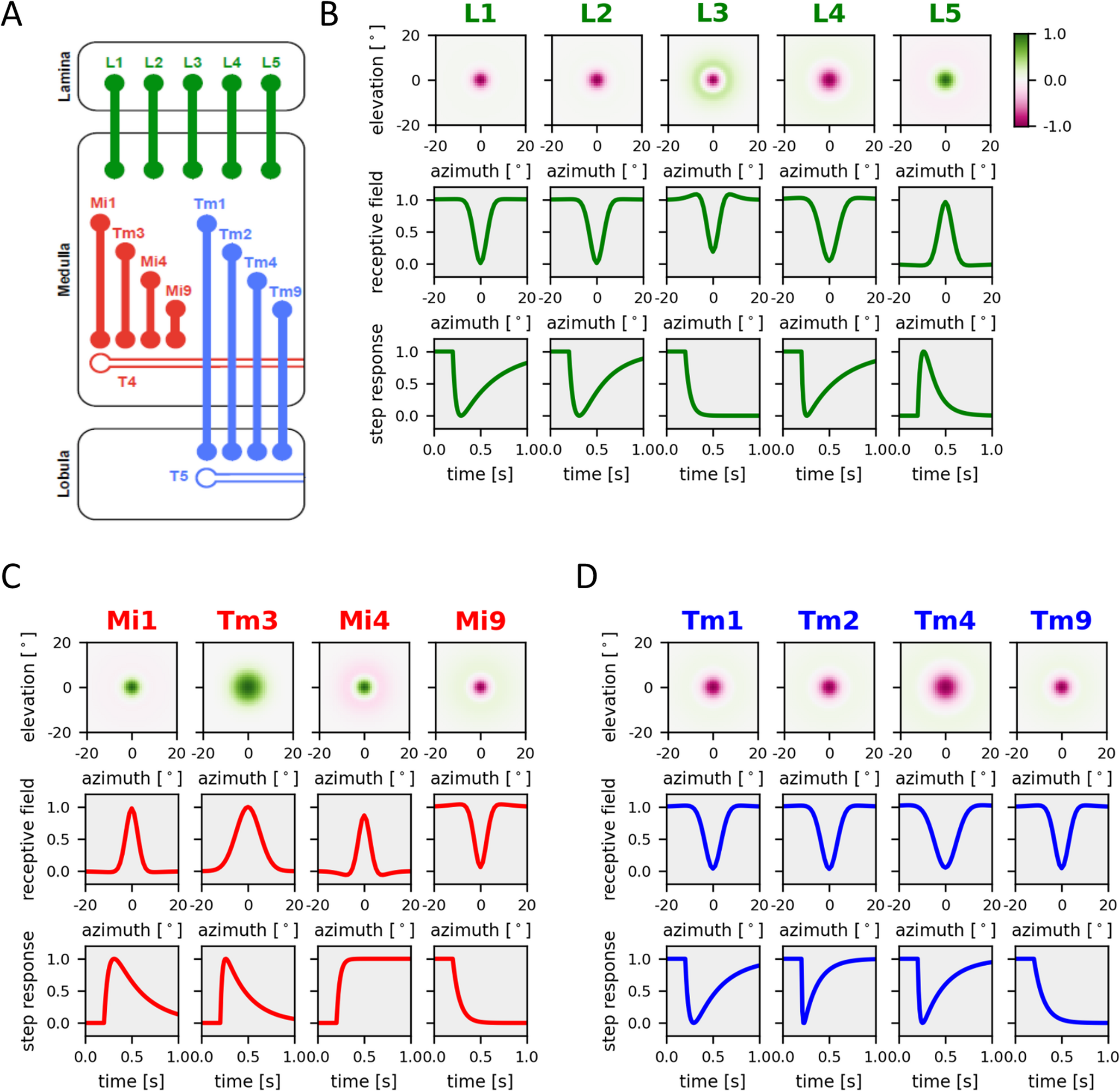
In a first round of simulations, I investigated to what extent all the different dynamics of fly visual interneurons can be accounted for using identical, uniform, passive membrane properties of all model neurons. Thus, the only way to achieve different response properties is by the network connectivity. The resulting receptive field properties from such simulations overall matched the experimental data in quite amazing detail, leading to a final cost of about 7% (Fig. 4). Importantly, the pronounced antagonistic surround of lamina neuron L3 and medulla neuron Mi4 was well captured by the model, indicating that inter-columnar connectivities can account for their spatial receptive field profiles. Furthermore, and of particular interest in the current context, the transient responses of lamina neurons L1, L2 and L4, as well as of medullar neurons Mi1, Tm3, Tm1, Tm2 and Tm4 were replicated by the model, together with the sustained responses of L3, Mi4, Mi9 and Tm9. However, unlike its biological counterpart, lamina neuron L5 responded in a sustained way. Furthermore, its response amplitude, as well as the one of medulla neuron Tm4, fell short of the respective measured amplitudes. As a final note, many responses showed ringing, indicating some sort of instability within feed-back loops.

Model simulation with electrically passive elements. Responses of model neurons (in red) with parameters optimized to fit experimental data (in gray). (A) Top: Spatial profiles of the receptive field of the five lamina cells L1-L5. Bottom: Temporal step response of the same neurons. (B) Same as A, but for columnar elements of the ON-pathway, Mi1, Tm3, Mi4 and Mi9. (C) Same as A, but for columnar elements of the OFF-pathway, Tm1, Tm2, Tm4 and Tm9

As a second step, I inserted an H-current into lamina neurons and minimized the cost, again starting from a random parameter set. This time, the model had 5 additional parameters determining the maximum conductance in each of the 5 lamina neurons and 3 parameters describing the voltage characteristics of the H-current, shared for all 5 lamina neurons. The resulting receptive field properties of the 13 selected neuron types were in most cases almost indistinguishable from the experimental data, with a final cost of only 3% (Fig. 5). As in the data, the spatial profiles of the receptive fields of lamina cell L3 and medulla neuron Mi4 had antagonistic surrounds, and that of medulla cell Tm3 was extending over several columns. The only significant deviation was seen in medulla neurons Tm3 and Tm4 where the model responses had a smaller amplitude than the real neurons. All other cells faithfully matched the data in their spatial profile as well as in their time-course. Furthermore, ringing was almost completely absent in the responses. Most importantly, the distinction between transient and sustained cells in the model was as clear as in the data.

Model simulation with H-current in L1, L2 and L5. Responses of model neurons (in red) with parameters optimized to fit experimental data (in gray). (A) Top: Spatial profiles of the receptive field of the five lamina cells L1-L5. Bottom: Temporal step response of the same neurons. (B) Same as A, but for columnar elements of the ON-pathway, Mi1, Tm3, Mi4 and Mi9. (C) Same as A, but for columnar elements of the OFF-pathway, Tm1, Tm2, Tm4 and Tm9

Next, I investigated to what extent the dynamic properties of this network still depend on the circuit connectivity or, alternatively, now are largely dependent on the intrinsic, transient membrane properties of lamina neurons L1, L2, L4 and L5. To this end, I switched off the H-current in the above network after optimizing the parameters with an H-current. This procedure led to a dramatic break-down of the match between model and data, quantified by a cost of more than 100% (Fig. 6). Importantly, all model neurons now responded in a sustained way, i.e., have lost their transient nature.

Model simulation with H-current shut off in L1, L2 and L5. Responses of model neurons (in red) after parameters optimized with H-current to fit experimental data (in gray). (A) Top: Spatial profiles of the receptive field of the five lamina cells L1-L5. Bottom: Temporal step response of the same neurons. (B) Same as A, but for columnar elements of the ON-pathway, Mi1, Tm3, Mi4 and Mi9. (C) Same as A, but for columnar elements of the OFF-pathway, Tm1, Tm2, Tm4 and Tm9

I finally tested the consistency of the above conclusions by comparing the parameter sets of the 10 best models obtained from 20 optimization runs in both scenarios, i.e., without and with an H-current. Without an H-current, final model costs ranged from 7% to about 11% (Fig. 7A), while costs of the 10 best models with an H-current all were found below 4% (Fig. 7B). This means that introduction of an H-current led to a cost reduction of about 50%. In each model category, parameters were highly correlated (Fig. 7C, D) indicating that different optimization runs converged on a similar parameter set each time. However, these parameter sets were significantly different for models without and with an H-current (Fig. 7E, F), with input and output gains being in general smaller for models without an H-current compared to models with an H-current. Interestingly, despite the fact that all five lamina cells were given an H-current, optimization consistently converged on models where only lamina cells L1 and L2 had a large maximum H-current conductance, a small one in lamina cells L4 and L5, and zero in lamina cell L3, which is in approximate agreement with the transcriptomic data of Davis et al. (2020).

Model Evaluation. Shown are the 10 best models from 20 optimization runs. (A, B) Remaining cost values of models without (A) and with (B) an H-current. (C, D) Correlation matrix showing the Pearson Correlation Coefficient of all parameters between each of the 10 models, without (C) and with (D) an H-current. (E, F) Average values +- variance of selected model parameters from the 10 best models without (E) and with (F) an H-current