2.1 Radiative transfer simulations2.1.1 Simulation setupFig. 1

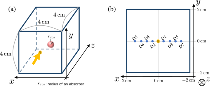
a Schematic image of the simulation box and coordinates. The pulse is perpendicularly injected from the center of the \(x-y\) plane (yellow point and arrow). The pulse (yellow point and arrow) is perpendicularly injected from the center of the \(x-y\) plane (\(z=0.0\,\textrm\) plane, i.e. the origin of the coordinates). A single spherical absorber with a radius \(r_\textrm\) is included in the simulation box. b Positions of the eight detectors. Each detector (blue point) is located along \(y=0.0\,\textrm\) on the pulse injected surface. The detectors are \(0.3\,\textrm\) apart from each other and the pulse injected point

In this study, we simulate pulse propagation in a cubic domain designed to model anomalies like brain hemorrhage and tumor near the brain surface and analyze the light emerging from the surface after undergoing multiple scattering and absorption. The simulation domain consists of a \(4.0\,\textrm \times 4.0\,\textrm \times 4.0\,\textrm\) cube and is discretized into \(128^3\) cells (Fig. 1). A single absorber, representing the anomaly, is placed within the domain and is assumed to have a spherical shape. For the simulations, we employ the radiative transfer code TRINITY [20], which accurately solves the RTE without relying on the diffusion approximation. Furthermore, recent enhancements by Abe et al. [29] have incorporated wavelet transformations into TRINITY, significantly improving computational efficiency. Using the updated TRINITY code, we compute the time evolution of the radiation field by numerically solving the following RTE

$$\begin&\frac)}\frac,\varvec)} + \varvec\cdot \varvecI(t,\varvec,\varvec) \nonumber \\&= -\)+\mu _s(\varvec)\}I(t,\varvec,\varvec) \\&\quad+ \mu _s(\varvec) \oint _ I(t,\varvec,\varvec')p(\varvec',\varvec) \textrm\varvec' \end$$

(1)

where t is time, \(\varvec\) is position, \(\varvec\) is direction (solid angle), \(v(\varvec)\) is the speed of light in the tissue, \(I(t,\varvec,\varvec)\) is the specific intensity, \(\mu _a(\varvec)\) and \(\mu _s(\varvec)\) are the absorption and scattering coefficients, respectively, and \(p(\varvec',\varvec)\) is a phase function. We assume a uniform refractive index of \(n=1.511\) throughout the domain, independent of the absorber properties, yielding a speed of light in tissue given by \(v=c/n\) where c is the speed of light in vacuum. The absorption coefficient \(\mu _a\) differs between the background tissue and the absorber. For background (i.e. no anomaly area), we set \(\mu _a=0.3\,\mathrm }\), while the absorber has ten times higher coefficient than the background (\(\mu _a=3.0\,\mathrm }\)). The scattering coefficient is fixed at \(\mu _s=80.0\,\mathrm }\) for both the background and the absorber [30, 31]. The phase function \(p(\varvec',\varvec)\) describes the angular redistribution of scattered light, characterizing the transition from the incoming direction \(\varvec'\) to outgoing direction \(\varvec\) at position \(\varvec\). For this study, we adopt the Henyey-Greenstein phase function:

$$\begin p(\varvec,\varvec') = \frac\frac'\cdot \varvec)^} \end$$

(2)

with an anisotropy factor of \(g=0.9\). The time evolution is computed from \(t=0\) to 3 nanoseconds (\(\textrm\)).

Fig. 2

Example snapshots of the photon energy density at \(t=0.5, \ 0.7, \ 0.9, \ 1.1\) nanoseconds (\(\textrm\)) on the \(y=2.0\,\textrm\) plane. The absorber is located at \((x, z)=(0.53, 1.34)\,\textrm\) with a radius of \(0.47\,\textrm\) and is indicated by the red circles. Due to the presence of the absorber, the energy density is reduced in its vicinity. The energy density is normalized by the maximum value at \(t=0.9\,\textrm\)

For the calculation of specific intensity in the time domain, we input the pulse used in Yajima et al. [20] from the center of a surface of the simulation box and eight detectors are set (see Fig. 1). Photons propagate through the simulation domain with undergoing scattering and absorption and are subsequently detected on the same surface where the pulse is injected. Figure 2 shows an example of the time evolution of the photon energy density on the \(y=0.0\,\textrm\) plane. Light injected at \(y=0.0\,\textrm\) propagates through the simulation box, undergoing multiple scattering and absorption events. The presence of a absorber reduces the local energy density around it. We arrange eight detectors (D1-8) along a horizontal line, each spaced \(0.3\,\textrm\) apart from both the pulse injection point and adjacent detectors, as illustrated in Fig. 1 (b). In detecting light signals, we adopt the same detector opening angle of \(\sim 15^\circ \) as in previous studies and obtain the signals in the same manner [20, 29]. Photons that go outside the simulation domain are not reintroduced into the system.

2.1.2 Specific intensity and absorption measure

For training our neural network, we first calculate the normalized intensity \(I_\textrm^i(t)\) at the i-th detector, defined as

$$\begin I_\textrm^i(t) = \frac^i(t)}^}}, \end$$

(3)

where \(I_\textrm^i(t)\) represents the intensity of the outgoing light toward the i-th detector in the case with an absorber as a function of time, while \(I_\textrm^}\) is the maximum intensity at the same detector when no absorber is present. Each intensity is estimated by integrating specific intensity over solid angles. Additionally, we calculate the absorption measure \(A^i(t)\) at the i-th detector, defined as

$$\begin A^i(t) = \frac^i(t)}^i(t)} - 1, \end$$

(4)

where \(I_\textrm^i(t)\) is the intensity detected at the i-th detector in the case without any absorber as a function of time. Since the absorption measure \(A^i(t)\) exhibits a more pronounced variation across the different absorber features compared to the normalized intensity \(I_\textrm^i(t)\), \(A^i(t)\) is considered to be more suitable for diagnostic purposes using our neural network [21]. We use both \(I_\textrm^i(t)\) and \(A^i(t)\) to train our neural network model.

2.1.3 Features in simulations

Due to the optical properties of the absorber and the simulation setup described above, the radiation field depends on the position and size of an absorber. Consequently, the light emerging from the surface of the simulation box is also a function of the position and size of the absorber. In this work, we run radiative transfer simulations using 640 different sets of the three features of the absorber for simplicity: horizontal direction \(x_\textrm\), depth \(z_\textrm\), and radius \(r_\textrm\), where \(x_\textrm\) and \(z_\textrm\) represent the center coordinates of the absorbers and we assume that absorbers are spherical with their centers located on the \(y=0.0\,\textrm\) plane. We note that, in this study, we intentionally restrict the absorber properties to these three features, although other factors, such as the vertical position \(y_\textrm\), the absorption coefficient \(\mu _\textrm\), the absorber shape, and the presence of multiple absorbers, can also significantly influence the temporal evolution of \(I_\textrm\) and A. Developing a neural network model that can rapidly and accurately infer time-resolved signals while accounting for all these factors is a highly challenging task, primarily due to the computational complexity of solving the RTE for a large parameter space. We therefore focus on this reduced set of features to establish a tractable and well-controlled framework, and extensions to include additional absorber properties will be explored in future work.

We randomly generate the sets of the features using the Latin hypercube sampling (LHS), which is a statistical technique that allows for the generation of a quasi-random set of parameter values from a multidimensional probability distribution [32, 33]. LHS is particularly suited for randomly sampling N parameter combinations from an M-dimensional parameter space with a small bias. The feature sets are generated as follows. First, we generate 640 pseudo-uniform random numbers from a 3D space, in which each variable is \(\in [0,1]\), using LHS. The numbers are then converted into the three features of absorbers following the inverse transform method. The radius \(r_\textrm\) is set so as to follow a continuous uniform distribution between \(0.1\,\textrm\) and \(0.5\,\textrm\). The horizontal direction \(x_\textrm\) follows a continuous uniform distribution between \(-2.0\,\textrm\) and \(2.0\,\textrm\) so that the absorber does not extend beyond the simulation box for a given radius \(r_\textrm\). For each value of \(r_\textrm\), the depth \(z_\textrm\) is sampled from a probability density function following a truncated exponential distribution, with values ranging between 0.7 and \(4.0\,\textrm\) to prevent the absorber from protruding beyond the box. For simplicity, we neglect the optical effect of the skull in our simulations since its optical properties do not differ significantly from those of brain tissue [34], although we consider the absorber to represent an anomaly site located behind the skull. For the exponential distribution, we choose the parameter of \(\lambda = 2.0\,\textrm\), which characterizes the scale length of the distribution and concentrates more absorbers at \(z \lesssim 2.0\,\textrm\). This choice is motivated by our observation that both the normalized intensity \(I_\textrm^i(t)\) and the absorption measure \(A^i(t)\) exhibit minimal sensitivity to absorbers located at \(z_\textrm \gtrsim 2.0\,\textrm\), while they vary more significantly when \(z_\textrm < 2.0\,\textrm\). Therefore, the neural network should focus on learning this sensitive region. Figure 3 shows the distribution of the features of the absorbers in the parameter space.

Fig. 3

Histograms (top) and scatter plots (bottom) of 640 sets of the features (horizontal direction \(x_\textrm\), depth \(z_\textrm\), and radius \(r_\textrm\)) used in our simulations. Each simulation includes a single absorber whose position and radius are determined by this distribution

Using the 640 sets of features, we perform simulations with a single absorber placed in the simulation box and obtain the optical values of \(I_\textrm^i(t)\) and \(A^i(t)\) at each detector.

2.2 Neural network2.2.1 Fully-connected neural network model

We employ the open-source python library PyTorch [35] to develop a neural network model that predicts the normalized intensity \(I_\textrm^i(t)\) and the absorption measure \(A^i(t)\) at each detector from a given set of the features of an absorber. Figure 4 illustrates the schematic image of our fully-connected neural network model, which employs deep multi-task learning. The network architecture consists of a single input layer, a shared hidden layer, and task-specific layers.

Fig. 4

Schematic image of our fully-connected neural network using deep multi-task learning. The input layer receives three absorber features: the horizontal position \(x_\textrm\), depth \(z_\textrm\), and radius \(r_\textrm\). The shared hidden layer and the three hidden layers in the task-specified layers have 32 neurons. The activation function for the shared layer is ReLU. The activation functions for the three hidden layers in the task-specific layers are Tanh. The output layers consist of \(N_\textrm^I = 254\) neurons for predicting the discrete-time evolution of the normalized intensity \(I_\textrm^i(t)\) and \(N_\textrm^A = 476\) neurons for the absorption measure \(A^i(t)\) at each detector (\(i = 1, \ldots , 8\))

The input layer of the network receives the three absorber features: the horizontal position \(x_\textrm\), depth \(z_\textrm\), and radius \(r_\textrm\). The shared hidden layer use the ReLU activation function. The task-specific layers contain three hidden layers, all using Tanh activation, and output layers. Each layer in the shared and task-specified layers has 32 neurons. The output layers consist of \(N_\textrm^I = 254\) neurons for predicting the discrete time evolution of \(I_\textrm^i(t)\) and \(N_\textrm^A = 476\) neurons for \(A^i(t)\). The weights in our network are initialized randomly following a Xavier normal distribution [36]. These weights are updated iteratively through forward and backward propagation to minimize the loss function, using the Adam optimizer [37] with a learning rate of 0.001. The training process involves 500 epochs, with a batch size of 8. Although we have run simulations from \(t=0\) to \(3\,\textrm\), we focus on partial time ranges around the peaks of \(I_\textrm^i(t)\) and \(A^i(t)\) since the peaks are strongly influenced by the features. Specifically, we employ the time ranges from \(t=0.4\) to \(1.2\,\textrm\) for \(I_\textrm^i(t)\) and from \(t=1.0\) to \(2.5\,\textrm\) for \(A^i(t)\). These time ranges correspond to the numbers of output dimensions of \(N_\textrm^I=254\) for \(I_\textrm^i(t)\) and \(N_\textrm^A=476\) for \(A^i(t)\), respectively. The loss function is computed as the sum of the mean squared error (MSE) of \(I_\textrm^i(t)\) and \(A^i(t)\), defined as

$$\begin MSE&= \sum _^8 \Biggl [ \frac^I} \sum _^^I} \left( I_\textrm^(t_j) - I_\textrm^(t_j) \right) ^2 \nonumber \\&\qquad \quad + \frac^A} \sum _^^A} \left( A^(t_j) - A^(t_j) \right) ^2 \Biggr ] \end$$

(5)

where the superscripts NN and true refer the values produced by our neural network and the true values, respectively.

2.2.2 Data for training, validation, and test

We train our network using two types of datasets: one without noise and another with added noise. The 640 datasets obtained from the simulations are first used for training and validation. To validate our neural network model, we perform k-fold cross-validation to determine the optimal network architecture and hyperparameters described above (e.g. number of neurons, learning rate, etc.). In this cross-validation, we employ \(k=5\), meaning that the datasets are randomly divided into 5 subsamples. One subsample is assigned as the validation set, while the remaining four are used for training. This process is repeated 5 times, with each subsample serving as the validation set once. For the noiseless data, we validate network architectures and hyperparameters straightforwardly following this cross-validation process. On the other hand, for the data with noise, we augment each training subsample tenfold through duplication and then add a Gaussian noise with a standard deviation of \(\sigma =0.01\) to the signals of \(I_\textrm^i(t)\) and \(A^i(t)\). We calculate the loss using Eq. 5 in each process at the 100th epoch for each fold. After testing various architectures and hyperparameter combinations, we find that both datasets yield the lowest average loss with the same network configuration. In addition, we find that incorporating the shared layer significantly improves the network performance, suggesting that this layer plays an important role in the prediction process. In the main results, we use the optimized neural network model to predict time-resolved signals. After finalizing the network architecture and the hyperparameters, we retrain the networks using all 640 datasets. The training processes take approximately 16 min for the network trained with noiseless data and 2.3 h for the network trained using data with noise on a single Intel Xeon Gold 6140 CPU core. We compare the performance of the network based on these different data handling methods.

For test data, we generate an additional 100 datasets by running radiative transfer simulations using feature sets that follow the same probability distribution as that used for the training data. The inference time of the trained machine learning model is approximately \(2\times 10^ \, \textrm\) when executed on a single Intel CPU. In the results section, we show the performance of our neural network model by comparing the signals predicted by our network with the true signals from the test data.