System design and specifications

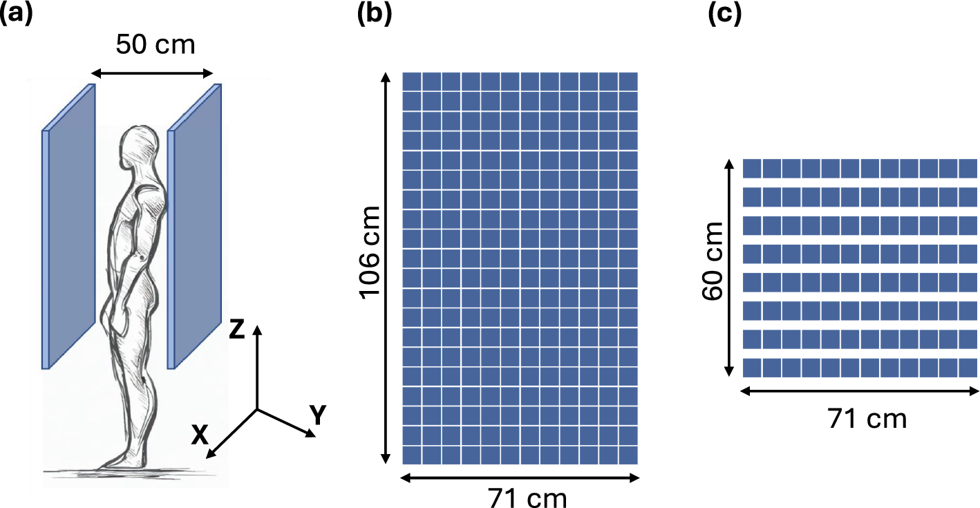
The L-FP, based on the original WT-PET design, consists of two flat panels placed 50 cm apart. Each panel has 20 rows of monolithic LYSO detectors of 50 × 50 × 16 mm3 with a 3-mm gap, bringing the AFOV to 106 cm. Horizontally, a width of 71 cm is achieved by placing 12 blocks of detectors with a gap of 10 mm between adjacent blocks. The sparse configuration of the WT-PET with reduced axial coverage, referred to as the SpM-FP in this work, features axially eight rows of detectors with 28-mm gaps between consecutive rows, achieving an AFOV of 60 cm. Each gap includes the initial 3-mm spacing plus an additional 25 mm, equivalent to half the size of a detector. This gap size of approximately half a detector width allows the extension of the AFOV while minimizing sensitivity loss and preserving image quality, as supported by a previous study [14]. Consequently, only limited panel motion is required to image the brain and torso, similar to the L-FP configuration. Schematic illustrations of the WT-PET concept and both configurations are shown in Fig. 1.

Fig. 1

a Schematic view of the WT-PET concept, b L-FP design, c SpM-FP design with 28-mm axial gaps and a reduced AFOV

The axial acceptance angle of the L-FP is 65° and reduced to 50° for the SpM-FP. We used a coincidence timing resolution of 300 ps full-width-at-half-maximum (FWHM), which we anticipate our system can achieve. The average spatial resolution of the LYSO monolithic detectors used for detector blurring is 1.14 mm FWHM parallel to the detector face and 2.67 mm FWHM along the depth as reported in [29] for measurements on the same detector.

Monte Carlo simulation and image reconstruction

We simulate the SpM-FP and L-FP designs using the Geant4 Application for Tomographic Emission (GATE) v9.2 [30] and evaluate their performance based on the NEMA NU 2–2018 protocol [31]. Table 1 summarizes the differences in system specifications and simulation parameters. The coincidence time window chosen for the SpM-FP and L-FP designs was 4 ns and 5 ns, respectively (calculated from the length of the most oblique LOR present in the system). The energy resolution was set to 11.5% for LYSO (455–645 keV window). The sources are simulated as 18F positrons, including the positron range and the physics of the non-collinearity. The exact gamma photon interaction time and position of the coincident events are recorded in the detector. The hits are grouped and saved as single events, and the coincidence sorting is done in GATE. No cut was applied to the axial acceptance angle.

Table 1 L-FP and SpM-FP design specifications and simulation parameters

To reconstruct the images of the simulated data, we use PETRecon, an iterative list-mode image reconstruction package developed locally and optimized for the WT-PET geometry. It is written in Julia, a high-level programming language for optimal GPU performance [32]. We reconstruct the true coincidences (511-keV photons originating from the same annihilation event and not scattered in the phantom) using the Maximum Likelihood Expectation Maximization (MLEM) algorithm (no subsets). We model the system’s timing and detector spatial resolution/DOI prior to reconstruction. The GATE simulation records the exact timestamps and interaction positions of the two coincident events. Before reconstruction, we blur these exact measurements by applying Gaussian kernels with FWHM values of 300 ps for time and 1.14 mm/2.67 mm for spatial coordinates, corresponding to the 2D intrinsic resolution and DOI, respectively. These values represent the average intrinsic performance of the monolithic detector. While this approach simplifies the actual behavior of such monolithic detectors, whose resolution typically worsens near the edges and varies with interaction depth, it provides a reasonable approximation. The accuracy of this homogeneous model is assessed in the spatial resolution study, which incorporates a spatially varying resolution model based on data from reference [29].

Phantom studies for performance evaluationSensitivity

The sensitivity of the SpM-FP and L-FP configurations was simulated using the NEMA standard 70-cm long line source placed at the center of the scanner and at 10-cm radial offset along two directions: parallel to the panels (X-axis) and towards the panels (Y-axis). To evaluate the axial sensitivity profile across a 106-cm AFOV for head and torso scanning, a 106-cm long line source was placed at the center. In the SpM-FP, the detector panels were moved vertically relative to the source to cover a scanning FOV of 106 cm, which was then extended by 15 cm at both the top and bottom, resulting in a total scanning FOV of 136 cm, as illustrated in Fig. 2. With the 15-cm extension on both ends, the head will be positioned at the center of the AFOV at the end of the scan, improving statistics for the brain region on one side and the pelvic area on the other. For comparison, the same source was also simulated in the L-FP.

Fig. 2

Schematic illustration showing the 106-cm line source simulated in the SpM-FP with upward panel motion to cover a scanning FOV of a 106 cm and b 136 cm (106 cm with an additional 15 cm at the top and bottom)

For both line sources, we use a 1-MBq 18F positron source in water surrounded by one to five concentric aluminum attenuating sleeves (2.5-mm thick) and extrapolate the results to find the attenuation-free system sensitivity. To simulate attenuation in a human body with a relatively low Body Mass Index (BMI), we surround the 106-cm line source with a 20-cm diameter water cylinder.

Spatial resolution

Twelve 18F positron point sources with a diameter of 0.5 mm were simulated to evaluate the system's spatial resolution following the NEMA protocol. Six sources were placed at the central transverse slice with offsets of 1, 10 and 20 cm along the X- and Y-axis and another repetition of the six sources at the transverse slice located at 3/8th of the AFOV. According to the NEMA standards, the voxel size of the reconstructed point source should not exceed one-third of the expected FWHM in all directions. Given the anticipated spatial resolution range of 1–2 mm, the images were reconstructed using a voxel size of 0.25 × 0.25 × 0.25 mm3. Since dual flat-panel systems measure incomplete data, filtered back-projection results in image artifacts. For a more realistic assessment of image resolution, the MLEM algorithm was used instead. To prevent artificial resolution enhancement caused by iterative reconstruction [33], all point sources were embedded in a warm background. The activity concentration ratio of point source to background was set to 160:1. Additionally, the source counts were subsampled prior to reconstruction to achieve a reconstructed point source-to-background contrast ratio between 0.1 and 0.2 [33]. For each source position, a minimum of 100,000 true coincidence events were used for image reconstruction. The background reconstruction was subtracted from the combined source and background reconstruction to generate the source-only image. The line profiles in all three directions of each source's point spread function (PSF) were drawn, and linear interpolation was performed to evaluate the FWHM. The reported values correspond to the 50th iteration, at which convergence in values was observed. These results incorporate a uniform model of the detector’s spatial resolution/DOI, based on a previous study of the same detector [29]. That study reported an average intrinsic 2D resolution of 1.14 mm across the entire detector and a DOI resolution of 2.67 mm over all six layers. The study also presented a 2D spatial resolution map showing a uniform resolution in the central 40 × 40 mm2 region, with degradation near the edges, extending as far as 5 mm from each edge. To assess the impact of this non-uniform detector resolution on system resolution, a spatially varying detector response function was implemented for an off-center point source. The function maintained a constant resolution of 1.02 mm in the central 40 × 40 mm2, increasing linearly to 1.35 mm at the edges, averaging out over the whole detector to the reported value of 1.14 mm.

Additionally, the model was also modified to include DOI resolution degradation in the two layers closest to the SiPM array. A constant DOI of 2.4 mm was used for layers 1 through 4, while 3.7 mm was applied to layers 5 and 6. These values were weighted according to the percentage of detected events in each layer, resulting in an average DOI resolution of 2.67 mm across the entire detector volume. The system resolution, expressed as FWHM, was evaluated using this spatially varying intrinsic resolution model and compared to the uniform resolution case for a point source simulated in the L-FP system at (10, 0, 0) cm.

Axial noise variability

To evaluate the axial noise variability along the AFOV of the sparse design due to the presence of gaps, a 3-min acquisition of a 20-cm diameter and 120-cm long water cylinder with a uniform 18F activity concentration of 3.7 kBq/ml was simulated [14]. The images were reconstructed with only true coincidences and a voxel size of 2 × 2 × 2 mm3. Attenuation correction and PSF modeling were implemented in the reconstruction. In the L-FP, only the LORs within the central 60-cm region of the AFOV were considered to enable comparison with the SpM-FP. A 16-cm diameter circular region of interest (ROI) was drawn on each slice, and the noise measure in each slice j was defined as:

where SDj and Cj are the standard deviation and average of the counts in each ROI, respectively.

Image quality

The NEMA image quality (IQ) phantom was used to evaluate the image quality of the SpM-FP design and compare it to that of the L-FP. It consists of six hot spheres of different diameters (10, 13, 17, 22, 28, and 37 mm) placed in a body phantom with a warm background and a cold lung insert. The sphere-to-background (STB) activity concentration ratio was 4:1, with a background activity of 5.3 kBq/ml and a 3-min acquisition of the phantom was simulated. The true coincidences were reconstructed with attenuation correction and PSF modeling and a voxel dimension of 2 × 2 × 2 mm3. To evaluate the contrast recovery in the presence of noise in the image, we used the same ROIs proposed by NEMA to compute the contrast-to-noise ratio (CNR) defined as:

where \(_\) is the average counts in ROI of sphere j, and \(_\) and \(_\) are the average and standard deviation of the counts in the background ROIs, respectively.

IQ body phantom with smaller spheres

A modified IQ phantom with small hot sphere sizes was simulated to probe the limits of the SpM-FP design in distinguishing small features (less than 12 mm in diameter). The overall geometry of the body phantom was kept the same, but the diameters of the hot spheres were reduced to 12, 10, 8, 6, 4 and 2 mm and simulated with a STB activity concentration ratio of 4:1 and 8:1 for a total acquisition time of 3 min. The images were reconstructed based on the true coincidences only, with a voxel size of 1 × 1 × 1 mm3, and the CNR was calculated for each sphere for an acquisition time ranging from 30 s to 3 min.

XCAT anthropomorphic phantoms

The anthropomorphic eXtended CArdiac-Torso (XCAT) phantoms are computational models of human anatomy designed for use across various imaging modalities to evaluate and optimize the imaging system performance [34]. In this study, a male XCAT phantom (BMI = 18.64) with an activity of 3 MBq/kg was simulated in both configurations, incorporating activity decay to represent imaging one hour after injection. The acquisition was simulated for 30 s on the L-FP and 120 s on the SpM-FP without further modeling of activity decay, given the relatively short simulation time. Attenuation and PSF modeling were implemented in the reconstruction with 2 × 2 × 2 mm3 voxels. Two 3-cm diameter 3D ROIs were placed in the liver and lung, and the normalized standard deviation was calculated for each. These values were plotted as a function of acquisition time for the SpM-FP and compared to the values for a 30-s acquisition with the L-FP.