MaskGraphene workflow

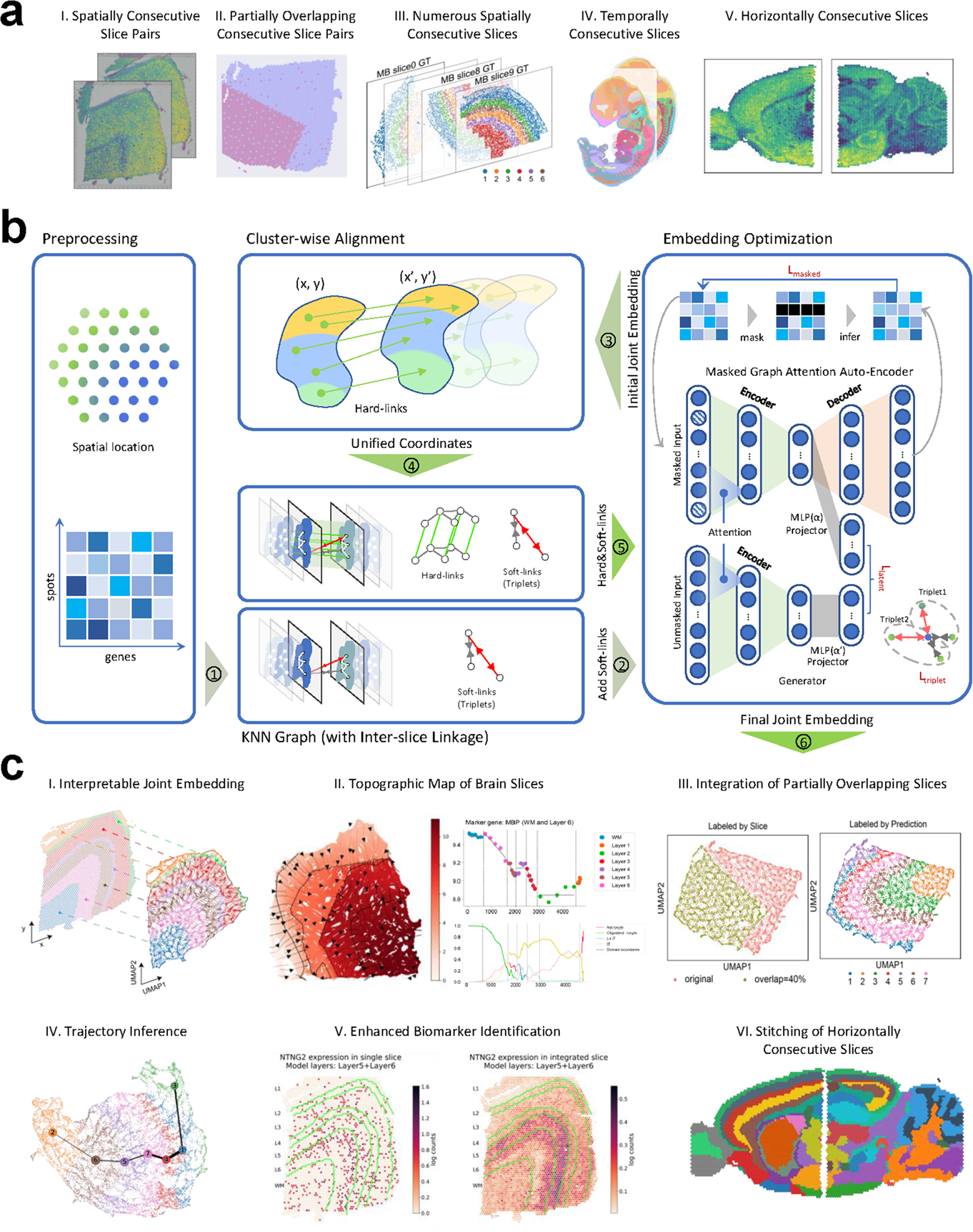
The MaskGraphene workflow (Fig. 1) takes as input a spot-gene expression matrix and spatial coordinates from two or more tissue slices. It begins with an initial integration using a masked graph attention autoencoder backbone with an intra-slice k-NN graph, jointly optimized with a masked self-supervised loss [36,37,38] and a triplet loss [27, 63] to identify shared clusters across slices. Triplet loss serves as “soft-links” in the latent space to strengthen inter-slice connections for initial integration. Next, cluster-wise local alignment is performed to establish “hard-links” (mappings) between slices, enabling all spots to be represented within a unified coordinate system. Using these unified coordinates, an inter-slice k-NN graph is constructed to model spatial relationships across slices. Finally, leveraging the same masked graph attention autoencoder architecture with the updated k-NN graph, MaskGraphene conducts a final integration step to optimize low-dimensional joint embeddings. Further details are provided in the corresponding sections below. With the final joint embeddings, MaskGraphene seamlessly integrates ST slices, enabling the identification of similar spatial domains or cell types across different tissue slices. We demonstrate MaskGraphene’s effectiveness through various quantitative and qualitative downstream analyses.

Initial integration (Steps 1-2)

As illustrated in Steps 1-2 of Fig. 1, MaskGraphene generates initial joint embeddings through an initial integration across spatial slices. Specifically, it employs a masked graph attention autoencoder to learn low-dimensional latent embeddings by jointly minimizing a masked self-supervised reconstruction loss and a triplet loss. Details of the graph model architecture, loss design, training strategy, and outputs of the initial integration are described in the subsections below.

Graph input processing

MaskGraphene processes gene expression data and spatial coordinates from two or more ST slices. First, it normalizes the total count of raw gene expressions and log-transforms them using the Scanpy package [44]. It then identifies the highly variable genes (HVGs) from all slices, and focuses on their HVGs intersection to maintain the consistency of expression features. For large-panel datasets (e.g., DLPFC, Stereo-seq), we select the top 5,000 HVGs to retain informative features while reducing noise. For small-panel datasets (e.g., MERFISH), we retain all genes to avoid discarding potentially critical information in low-dimensional settings.

Graph model backbone

In this section, we present the mathematical formulation and details of our backbone, the graph attention autoencoder. This model comprises five main components: the encoder, graph attention mechanism, decoder, projector, and generator.

Encoder. The encoder generates node (spot) embeddings by aggregating information from all neighbors. We denote \(\textbf_u^\) as the feature of spot u. In the masked graph modeling framework used in MaskGraphene, a subset of these node features is intentionally masked to enable self-supervised reconstruction, encouraging the encoder to capture context-aware representations. The specific masking strategy is described in the following section. The \(l^}\) encoder layer generates the embedding of spot u in layer l as follows:

$$\begin \textbf^_u = \epsilon \left( \sum \limits __u} \alpha ^_ (\textbf^ \textbf_v^)\right) \end$$

(1)

where \(\alpha ^_\) is the attention coefficient, discussed further below, \(\epsilon\) is the activation function, \(\mathcal _u\) denotes all the neighbors of node u including u itself, \(\textbf_^\) denotes the embedding of node v in the \(l-1\) layer, and \(\textbf^\) is the matrix of trainable parameters in \(l^\text \) layer.

Graph attention mechanism. The attention coefficient \(\alpha _^\) is calculated by (2) and (3) where \(\oplus\) is the concatenation operation and \(\sigma\) is a sigmoid activation function.

$$\begin \alpha ^_=\frac^^}}_^))})} \in \mathcal _}\exp ^^}}_}^))}} \end$$

(2)

$$\begin }^_ = \textbf^\textbf_^ \oplus \textbf^\textbf_^ \end$$

(3)

where \(\textbf^\) is another learnable parameter. The attention mechanism here is exploited to strengthen the connection between nodes that are represented by similar expression profiles. The attention coefficient \(\alpha ^_\) indicates the different contributions of each neighbor used in the aggregation process. The weights of edges are automatically calculated, based on node embedding.

Decoder. The decoder attempts to reconstruct the normalized expression profile for each spot u given the latent embeddings of the encoder. The \(l^}\) layer of the decoder (from the perspective of spot u) defined as:

$$\begin \hat}^_u = \epsilon \left( \sum \limits __u} \hat^_ (\hat}^ \hat}_v^)\right) \end$$

(4)

where \(\hat^_\) is the decoder attention coefficient which is calculated similarly as \(\alpha ^_\) in the encoder, and \(\hat}^\) is the matrix of trainable parameters in \(l^\text \) layer.

The reconstruction loss function is introduced in the next Methods section in the context of masked self-supervised loss.

Projector. The projector is a multi-layer perceptron (MLP) serving as the decoder for input feature reconstruction. It consists of two layers that map the latent space to the representation space for prediction.

$$\begin \bar} = (\textbf) \end$$

(5)

where \(\textbf\) denotes the latent embedding of encoder from either a masked or an unmasked graph in MaskGraphene, as illustrated in Fig. 1, and \(\bar}\) denotes the output of projector.

Generator. The generator has an identical structure to the aforementioned encoder and projector but with a different set of trainable parameters \(\xi _\) and \(\xi _\). It works on the unmasked graph input to produce the latent target representation \(\bar}\), which is leveraged to train the encoder and projector network to match the output of the generator on masked nodes.

$$\begin \bar} = Projector(Encoder(\textbf,\textbf; \xi _); \xi _) \end$$

(6)

where \(\textbf\) and \(\textbf\) denote the adjacency matrix and input node features of the unmasked graph.

We currently employ a symmetric encoder structure of 512, 32 (and 32, 512 for the decoder) in the MaskGraphene model. Detailed grid search results for the sensitivity analysis are provided in Additional file 1: Note S2 and Fig. S33.

Masked self-supervised reconstruction loss

For our graph model backbone, we introduced a self-supervised loss to reconstruct the node features that are randomly masked from the input gene expression matrix.

Specifically, MaskGraphene perturbs the input graph by masking node features and then attempts to reconstruct the original input. A subset of input spots is randomly selected, and their expression profiles are set to zero. A re-mask decoding strategy is also adopted, in which the latent embeddings of masked nodes are stochastically re-masked prior to decoding. The masking and re-masking rates are empirically set to 0.1/0.1 or 0.5/0.5 for the two dataset types (see Additional file 1: Note S2 and Fig. S34 for details and sensitivity analysis). This strategy aims to enforce the reconstruction in the embedding space and regularize the node feature reconstruction.

For each node \(i\), let \(\textbf_i\) represent its reconstructed gene expression via the decoder. The reconstruction loss function is formulated as:

$$\begin \mathcal _} = \frac|}\sum \limits _} \left( 1 - \frac_}^\textbf_}}_}|| \cdot ||\textbf_}||} \right) ^\mathbf , \mathbf \ge 1, \end$$

(7)

where \(\textbf_i\) denotes the original normalized expression profile for spot i, \(\bar\) is the subset of spots with masked features in the graph, and \(\gamma\) is a scaling factor for adjusting loss (empirically set to 1; see Additional file 1: Note S2 and Fig. S35 for sensitivity analysis). Using this scaled cosine error loss to measure the reconstruction error, the model learns node embeddings within a masked autoencoder framework.

To further leverage the feature information, a supporting network is utilized as the target generator to produce latent prediction targets from the unmasked graph. This generator, as previously described, shares the same structure as the aforementioned encoder and projector but operates with a different set of trainable parameters. MaskGraphene simultaneously optimizes the parameters of the encoder, projector, and generator by minimizing the following loss function:

$$\begin \mathcal _} = \frac\sum \limits _^ \left( 1 - \frac}_}^\bar}_}}}_}|| \cdot ||\bar}_}||} \right) ^\mathbf , \mathbf \ge 1, \end$$

(8)

where N denotes all the spots in the unmasked graph, \(\bar}_\) represents the output of projector from the masked graph, and \(\bar}_\) denotes the output latent targets of generator from the unmasked graph.

MaskGraphene simultaneously optimizes two objective functions with a balancing coefficient \(\lambda\) (empirically set to 1; see Additional file 1: Note S2 and Fig. S35 for sensitivity analysis):

$$\begin \mathcal _} = \mathcal _} + \lambda \mathcal _} \end$$

(9)

The intuition behind this loss design is to prevent the network from oversmoothing singular yet biologically critical features in the gene expression profiles, while simultaneously suppressing noise from batch effects and other technical artifacts. Such masking could lead to ambiguity between real and artificially masked zeros. However, our framework incorporates an auxiliary network (the generator and projector components described in the network structure) that processes the unmasked expression data and its corresponding embeddings. This auxiliary branch contributes to the joint optimization through the latent loss and helps regularize the learning process, providing the model with access to the true data distribution. As a result, even though the main network operates on masked input (with zeros as placeholders), the auxiliary network helps guide the learning dynamics and mitigates potential confusion arising from the sparsity. This dual-network design offers a practical balance between effective masking and accurate optimization in sparse settings.

Triplet loss

To learn the initial joint embeddings in the graph model, MaskGraphene leverages “soft-links” to enforce local geometric structure preservation among spots across slices and enhance inter-slice connections.

For “soft-links”, MaskGraphene employs mutual nearest neighbors (MNNs) [64] from each pair of consecutive slices to dynamically construct spot triplets based on their embeddings during training. The inter-slice connections, denoted as “soft-links”, differ from “hard-links” - introduced in Step 3 of the alignment and incorporated in Steps 4-5 of the final integration - in that they are not directly integrated into the k-NN graph. Instead, they are reinforced through the triplet loss, a method often used in single-cell RNA-seq batch correction [27, 63]. These “soft-links” are designed to emphasize differences between dissimilar spots across slices while clustering similar spots closer together. The objective is to bring similar spots nearer and separate contrasting ones [63].

In detail, triplet loss is based on the idea of triplets, which consist of an anchor spot \(\textbf\), a positive spot \(\textbf\), and a negative spot \(\textbf\). For each triplet \((\textbf, \textbf, \textbf)\), the loss is defined as follows:

$$\begin \mathcal _} = \max \left( (\textbf, \textbf) - (\textbf, \textbf) + \alpha , 0\right) \end$$

(10)

where \((\textbf, \textbf)\) is the Euclidean distance between the anchor spot \(\textbf\) and the positive spot \(\textbf\), measured in the joint embedding space, \((\textbf, \textbf)\) is the distance between the anchor spot \(\textbf\) and the negative spot \(\textbf\), \(\alpha\) is a margin that controls the minimum difference required between the distances of similar and dissimilar pairs. To construct triplets, we first determine MNNs across two slices. MNNs are constructed by taking the pairs of spots from distinct slices that are mutually k-nearest-neighbors [65] in the joint embedding space. After we identify MNNs matches between two slices, we define each MNN match as the \((\textbf, \textbf)\) pair. We further take each spot from MNN matches of one slice as an anchor spot and randomly select any spot from the other slice as a negative spot to form the \((\textbf, \textbf)\) pair. An alternating optimization strategy is adopted to optimize triplet loss. Specifically, every 100 training epochs (during which the model is primarily minimizing the masked self-supervised reconstruction loss), we recompute the triplets using the most recent low-dimensional embeddings. This updated triplet set better reflects the current embedding space and allows the triplet loss to be further minimized. This iterative process ensures that the triplet loss remains relevant throughout training and helps improve the alignment and integration of spatial slices. Triplet loss encourages the model to pull the anchor and positive spots (MNNs across slices) closer in the embedding space while pushing the anchor and negative spots (dissimilar spots across slices) farther apart.

Training strategy

During training, MaskGraphene adopts a two-phase optimization strategy to ensure stable convergence and robust embedding learning. In the first phase, all components of the model, including the encoder, projector, generator, and decoder, are trained jointly using backpropagation and a shared optimizer (e.g., Adam). This joint training enables the different modules to co-adapt effectively. The model is optimized using a combination of masked reconstruction loss and latent loss. The masked loss encourages accurate recovery of missing gene expression values under partial feature masking, using a scaled cosine error to handle variations in feature magnitude. At the same time, the latent loss enforces consistency between the encoder and projector outputs by minimizing the difference between latent representations from raw and masked inputs. This helps stabilize the embedding space and prevents collapse. After the model learns a stable embedding, we enter the second phase and introduce a triplet loss over soft-links. This loss pulls similar spots closer and pushes dissimilar ones apart, refining the embedding space to better preserve spatial structure and improve cross-slice alignment. Delaying the triplet loss until after initial convergence avoids early-stage instability and enables more effective metric learning.

Outputs of initial integration

After training the masked graph attention network with soft-links, we obtain joint spot embeddings across all slices. These embeddings are then used to perform joint clustering using mclust [48], yielding the initial clustering output. These initial embeddings, though sufficient for defining shared clusters across slices, are not yet fully optimized for spatial accuracy. They serve as a starting point for the next step - cluster-wise local alignment - which produces hard-links that refine inter-slice relationships and lead to a second round of embedding optimization.

Cluster-wise local alignment to generate “hard-links” (Step 3)

After identifying shared clusters across slices - each representing a common tissue domain - as illustrated in Step 3 of Fig. 1, we perform cluster-wise local alignment to establish direct correspondences (hard-links) between spots across slices. Rather than conducting a global alignment across all spots, which can be computationally intensive for large-scale datasets, we restrict alignment to spots within matched clusters. This localized strategy enhances computational efficiency and reduces false positive mappings, particularly in cases where slices are only partially overlapping or not perfectly adjacent along the z-axis. Details of the local alignment method are described in the subsections below.

Spot-to-spot mapping

To enhance inter-slice connections, we developed a cluster-wise optimal transport (OT)-based local alignment method to establish reliable spot-to-spot (node-to-node) mapping (alignment) across slices, enabling the unification of all spots into a shared coordinate system for constructing the inter-slice k-NN graph in MaskGraphene’s graph model during Steps 4-5 of the final integration. This cluster-wise alignment process begins with the previous initial integration step, which performs joint clustering to identify shared clusters across slices. Once shared clusters are identified across slices, cluster-wise OT-based local alignment is performed. Specifically, for each pair of shared clusters (representing the same domain across each pair of slices), following prior work on spatial slice alignment (e.g., PASTE [31]), we adopt a standard Gromov-Wasserstein optimal transport (GW-OT) formulation to compute probabilistic couplings between spots and derive spot-to-spot mappings. Unlike PASTE, which solves a single global fused GW problem per adjacent slice pair, MaskGraphene solves multiple cluster-wise GW problems over matched domains across all slices. Aggregating these local alignments provides global context while improving robustness to partial overlap and localized deformations. Each cluster-wise GW problem is optimized with an iterative conditional gradient method [66].

A detailed description of the problem is provided in Additional file 1: Methods S1. Given H slices that have \(M\) shared clusters identified from the initial clustering, the complete mapping (alignment) \(\Pi ^h\) between the two slices h and \(h+1\) is obtained by combining the transport plans (weights) across all clusters, with spots ordered according to their cluster labels:

$$\begin \Pi ^h = \left[ \begin \Pi ^ & 0 & 0 & \cdots & 0 & \cdots & 0 \\ 0 & \Pi ^ & 0 & \cdots & 0 & \cdots & 0 \\ 0 & 0 & \cdots & \Pi ^ & \cdots & 0 & 0 \\ \vdots & \vdots & \cdots & \vdots & \cdots & \vdots & \vdots \\ 0 & 0 & 0 & \cdots & 0 & \cdots & \Pi ^ \end\right] , \end$$

(11)

where \(\Pi ^ = [\pi ^_]\) is the transport plan (weight) between slices \(h\) and \(h+1\) in cluster \(m\). By deriving shared clusters from an initial integration of all slices and assembling \(\Pi\) from multiple small, cluster-wise GW problems (across all adjacent slice pairs), our local mapping is globally informed by the entire set of slices.

Coordinate system unification

After obtaining the transport weights (spot-to-spot mapping) for all clusters, referred to as “hard-links”, MaskGraphene integrates these inter-slice connections into its final k-NN graph model by employing three distinct strategies, each designed for specific integration scenarios.

Firstly, when the two slices \((X, D, g)\) and \((X', D', g')\) are adjacent consecutive slices and are used for pairwise integration (e.g., pairwise DLPFC, MHypo, and breast cancer slices sampled along the z-axis; or mouse and Drosophila embryo slices at closely matched developmental stages, as in this study.), we project the second slice to the same coordinate system as the first slice after we find the mappings \(\Pi\). The following generalized weighted Procrustes problem is solved to apply for coordinate transformation [31]:

$$\begin \hat, \hat = \min _^, v \in \mathbb ^2, R^T R = I} \sum \limits _ \pi _ \Vert z_ - Rz_' - v \Vert ^2, \end$$

(12)

where \(\hat\) is the rotation matrix and \(\hat\) is the translation vector.

The updated spatial coordinates of spot \(j\) in slice \((X', D', g')\) are then given by:

$$\begin \hat_' = \hat z_' + \hat. \end$$

(13)

Secondly, when multiple (>2) consecutive ST slices (e.g., DLPFC four-slice, MHypo five-slice, MB ten-slice, and mouse embryo six-slice integration in this study) are available for integration, achieving a robust unified coordinate system across all slices becomes increasingly challenging, particularly as the number of slices grows and geometric similarity between slices diminishes, with some adjacent slices exhibiting only partial overlap. MaskGraphene addresses this challenge by employing two alternative strategies: (1) coordinate replacement and (2) coordinate transformation, both designed to unify the coordinate system across slices. As shown in our results for the DLPFC, MHypo, and MB multi-slice integration, both strategies perform comparably well. Users may choose either strategy; however, for integration involving a large number of slices (e.g., >10), we recommend using coordinate transformation for greater robustness.

(1) Coordinate replacement via hard-links (by default): in this approach, we first compute spot-to-spot correspondences for all adjacent pairs of slices (1-2, 2-3, ...) using our cluster-wise local alignment, which outputs transport plans (weights) \(\Pi\) reflecting both spatial proximity and transcriptional similarity. For each spot in slice \(i+1\), we define its highest-confidence counterpart in slice i as the match with the largest normalized OT transport weight. After obtaining these highest-confidence mappings for all adjacent pairs, we perform a backward sweep from the last slice to the first. At each step, we replace every spot’s coordinates in slice i with those of its highest-confidence counterpart in slice \(i-1\). Because earlier slices have already been updated in prior steps, these replacements are recursively composed, ensuring that, by the end of the sweep, all slices are expressed in the coordinate system of slice 1. This cascading update strategy preserves local geometric accuracy while reducing error accumulation, enabling efficient construction of a multi-slice k-NN graph that integrates both intraslice and inter-slice connections without requiring any additional global transformations.

(2) Coordinate transformation via optimization: building on the local shared clusters (domains) identified during initial integration, we perform spatial coordinate transformation across multiple slices by predicting their coordinate systems using a mutual nearest neighbor (MNN) graph constructed from the unified spatial coordinates of the spots. The process is framed as an optimization problem guided by an objective function [33]. To address partially overlapping slices during multi-slice integration, a penalty term is incorporated to account for the proportion of overlapping spots. Using the differential evolution optimization algorithm [67], we determine the optimal transformation parameters - including translation vectors and rotation angles - for each slice. These parameters are then used to transform the coordinates of each slice. A detailed description of the optimization problem is provided in Additional file 1: Methods S2.

In summary, for multi-slice integration, users can select either coordinate replacement or coordinate transformation to unify the coordinate system across slices. In our study, both methods exhibited comparable performance overall; however, coordinate transformation demonstrated superior results for MB ten-slice integration.

Thirdly, when horizontally consecutive slices are integrated (e.g. mouse brain sagittal sections divided into anterior and posterior portions in this study), “hard-links” are directly incorporated as edges in the k-NN graph to strengthen inter-slice connections. Coordinate transformation or replacement is unnecessary, as these slices are horizontally connected. Subsequently, the final k-NN graph, incorporating both intraslice and inter-slice connections, is constructed.

It is worth noting that MaskGraphenes allows users to also utilize other state-of-the-art alignment tools to generate transport weights (spot-to-spot mappings) and unify coordinates across slices.

Final embedding optimization (Steps 4-5)

After performing cluster-wise local alignment, we generate hard-links between slices and unify their coordinate systems. These alignment-derived connections are considered hard-links because they are explicitly added as inter-slice edges in the k-NN graph. We then retrain the masked graph attention network using both the hard-links (from alignment) and soft-links (from the triplet loss) to carry out the final integration. This process yields the final joint embeddings across slices, as illustrated in Fig. 1. By incorporating alignment-based hard-links, we strengthen inter-slice connectivity and enable the model to better preserve the underlying geometric structure across slices, thereby enhancing the overall integration quality. These final joint embeddings can then be leveraged for a variety of downstream analyses.

In constructing the k-NN graph, we adopt an empirical strategy to determine the number of neighbors k. Specifically, we fix the within-slice k to 6 for all datasets, and set \(k=15\) when performing coordinate unification across slices. To assess sensitivity, we conducted a grid search over a range of k values and observed that the model performance remained largely consistent, demonstrating its robustness to this hyperparameter choice.

The primary distinction between the initial and final joint embeddings lies in the incorporation of hard links into the k-NN graph during the latter stage. The initial embeddings are generated to facilitate shared cluster/domain identification across slices, serving as a foundation for cluster-wise local alignment. Thus, the main objective of the initial integration is to enhance domain detection through joint embedding. In contrast, the final integration step further refines the joint embeddings by explicitly incorporating spatial hard links, aiming to preserve the original geometric structure for improved interpretability.

As detailed in Additional file 1: Note S1 and Figs. S36-S37, we compared the initial and final embeddings, and further benchmarked the initial embeddings against those from STAligner. In MaskGraphene, the initial embeddings are generated using slice-specific k-NN graphs combined with a triplet loss, aligning with the foundational strategy adopted by ST integration methods such as STAligner. This evaluation underscores the added benefit of the masking mechanism in our graph model for cross-slice domain identification. Our results showed that the initial embeddings outperformed STAligner in clustering performance, as measured by ARI, across both pairwise and multi-slice integration tasks. This performance was further enhanced by the final embeddings. Overall, the final embeddings demonstrated the highest quality in terms of iLISI, Isometry correlation, and Procrustes dissimilarity, followed by the initial embeddings and then STAligner.

Ablation study design and model variants

To assess the contribution of each component in MaskGraphene, we performed a comprehensive ablation study by systematically modifying the model’s architecture and loss functions. The full model, referred to as MaskGraphene-Full, integrates four key modules: a) a graph encoder utilizing hard inter-slice links to capture geometric priors, b) a masked reconstruction loss to support self-supervised feature learning, c) a triplet loss to enforce soft similarity constraints across slices, and d) a latent regularization loss to improve stability and generalization. This configuration served as the reference for all comparisons.

To isolate the role of each component, we constructed the following model variants (summarized in Additional file 1: Table S3): (1) MaskGraphene-MLP: A baseline that removes all graph-based operations and the masking strategy. It employs a simple multilayer perceptron (MLP) to process the input features and retains only the reconstruction and triplet losses. This variant evaluates the performance of a purely feature-based model without spatial priors or self-supervised regularization. (2) MaskGraphene-GAE: A graph autoencoder variant that retains the hard-link graph structure and the triplet loss but excludes the masked reconstruction mechanism. Since the latent loss is designed to work in conjunction with masked features, it is also removed. This variant isolates the contribution of geometric encoding without the self-supervised masking framework. (3) MaskGraphene-HardlinkOnly (NoTriplet): This variant removes the triplet loss, thereby eliminating soft similarity-based alignment across slices. It retains hard-links, masked reconstruction loss, and latent loss. This setup evaluates whether rigid structural priors alone are sufficient for achieving meaningful alignment. (4) MaskGraphene-MaskOnly (NoAuxLoss): This model retains the masked reconstruction and the graph encoder but omits both the triplet loss and latent loss. It serves to examine whether masked modeling alone, in the absence of auxiliary guidance, can support robust integration. For model variants (1) - (4), the initial integration and alignment steps were kept identical to those of the full model to ensure that the hard-links remained unchanged, even not used at all. (5) MaskGraphene-SoftlinkOnly: This configuration eliminates hard inter-slice links in the final embedding optimization steps, relying solely on soft similarity constraints introduced by the triplet loss. It retains the masked reconstruction and latent loss components. This variant tests whether soft-links, without explicit spatial priors, can guide effective integration across slices.

All models were trained using the same pipeline and hyperparameters to ensure fair comparison. We evaluated each variant using a comprehensive suite of quantitative and qualitative metrics, including layer-wise alignment accuracy, spot-to-spot matching ratio, iLISI, Isometry correlation, Procrustes dissimilarity, and UMAP visualizations. This ablation framework enables a fine-grained analysis of the role played by masking strategies, graph structure, and auxiliary objectives in achieving accurate, interpretable, and spatially coherent integration of multi-slice ST data.

Random seed analysis

The graph model is non-deterministic and may exhibit variance, especially in clustering outcomes. To generate Adjusted Rand Index (ARI) values for clustering performance, we fixed the random seeds in MaskGraphene for all datasets. For tools that do not fix seeds, such as STAligner and DeepST, we selected the best ARI value from 10 runs for each experiment. Additionally, we evaluated the robustness of all tools by varying the random seed and performing 20 iterations for each integration experiment, with ARI box plots illustrating the results. As shown in Additional file 1: Fig. S38, MaskGraphene consistently outperformed other tools across nearly all integration scenarios, highlighting its robustness.

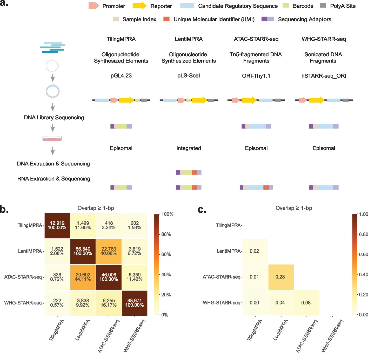
Benchmark datasets

We employed seven ST datasets with a total of 53 slices for benchmarking, which had corresponding manual annotations shown in Additional file 1: Table S1.

Specifically, (1) the human DLPFC (dorsolateral prefrontal cortex) dataset, generated with 10x Visium, includes 12 human DLPFC sections with manual annotation, indicating cortical layers 1 to 6 and white matter (WM), taken from three individual samples [39]. Each sample contains four consecutive slices (for example, slice A, B, C, and D in order). In each sample, the initial pair of slices, AB, and the final pair, CD, are directly adjacent (10\(\mu\)m apart), whereas the intermediate pair, BC, is situated 300\(\mu\)m apart. The number of spots ranges from 3,431 to 4,788, with a total of 33,538 expressed genes across all slices.

(2) The MHypo (mouse hypothalamus) dataset by MERFISH contains five manually annotated consecutive slices [23] labeled Bregma -0.04mm (5,488 cells), Bregma -0.09mm (5,557 cells), Bregma -0.14mm (5,926 cells), Bregma -0.19mm (5,803 cells), and Bregma -0.24mm (5,543 cells). Expression measurements were taken for a common set of 155 genes. Each tissue slice includes a detailed cell annotation, identifying eight structures: third ventricle (V3), bed nuclei of the stria terminalis (BST), columns of the fornix (fx), medial preoptic area (MPA), medial preoptic nucleus (MPN), periventricular hypothalamic nucleus (PV), paraventricular hypothalamic nucleus (PVH), and paraventricular nucleus of the thalamus (PVT).

(3) The MB (mouse brain) dataset [33, 49] by MERFISH has a total of 33 consecutive mouse primary motor cortex tissue slices with similar shapes, which can be used for 3D reconstruction. We selected the first 10 consecutive slices for benchmarking in this study. Region annotations include the six layers (L1-L6) and white matter (WM). The number of spots ranges from 2,033 to 5,624, with a total of 254 expressed genes.

(4) The dataset of mouse brain sagittal sections (MB2SA&P), generated with 10x Visium, includes two slices of the anterior and posterior mouse brain. The number of spots is 2,695 and 3,353 for two slices, respectively, with both containing 32,285 expressed genes. Only the anterior section includes annotations [13, 50].

(5) The mouse embryo dataset by Stereo-seq has over 50 slices, and the slices at time points E11.5 to E16.5 were used in our experiments. The number of spots is 30,124 and 51,365 for slices E11.5 and E12.5, respectively, with 26,854 and 27,810 captured and expressed genes. In total, these six slices contain 496,494 spots. These data are from a large stereo-seq project called MOSTA [15]: Mouse Organogenesis Spatiotemporal Transcriptomic Atlas by BGI.

(6) The 10x Visium dataset for human breast cancer from the 10x Genomics database contains two slices with approximately 3,800 spots and 36,000 genes. Manual annotations are available for one slice, defining 20 regions, including DCIS/LCIS, healthy tissue, invasive ductal carcinoma (IDC), and low-grade tumor margins [68]. We applied our local alignment module to align spots across the two slices and transferred domain labels from the annotated slice to the second slice.

(7) The Drosophila embryo dataset by Stereo-seq comprises 16 slices [47]. In the original study, Stereo-seq was applied to spatially profile gene expression in Drosophila melanogaster across multiple developmental stages, including two late-stage embryos (14-16 hours and 16-18 hours after egg laying, denoted E14-16 and E16-18) and three larval stages (L1, L2, and L3). Each spatial slice contains approximately 1,000 spots, with a median of \(\sim 2\),000 unique molecular identifiers (UMIs) per spot. Cell type annotations were obtained through unsupervised clustering of gene expression profiles, followed by manual labeling using known marker genes.

Simulated datasets

Due to the limited availability of benchmark datasets for evaluating spot-to-spot alignment accuracy, we employed our recent ST simulation method [16] to generate five simulated 10x Visium datasets for this purpose. Specifically, we used the DLPFC 151673 slice as the reference and created new slices by altering the spatial coordinates of the reference through rotation. To further simulate real-world scenarios, we adjusted the number of spots in each slice by removing spots that no longer aligned with the grid coordinates after rotation. To preserve the fidelity of real 10x Visium data, we arranged the tissue spots in a hexagonal grid pattern rather than a rectangular one. By applying rotations with different degrees, we generated slices with varying overlap ratios (20%, 40%, 60%, 80%, and 100%) relative to the reference slice.

Quantitative metrics Adjusted Rand Index (ARI).

ARI measures the similarity between two data clusterings by assessing the concordance of pairwise data point groupings. It evaluates whether pairs of points are assigned to the same cluster or different clusters in the two clusterings. The ARI ranges from -1 to 1, where 1 represents perfect agreement, 0 indicates clustering that is no better than random, and negative values suggest disagreement between the clusterings.

Layer-wise alignment accuracy.

This metric [16] is based on the hypothesis that aligned spots from adjacent consecutive slices are likely to belong to the same spatial domain or cell type. Joint spot embeddings from each method are used to align (anchor) spots from the first slice to corresponding (aligned) spots on the second slice for each slice pair. Spot proximity for alignment is determined using Euclidean distance. Alignment accuracy is calculated as the proportion of anchor spots in the first slice that are aligned to spots in the second slice belonging to the same spatial domain or cell type. For the DLPFC slices, which exhibit a unique layered structure, this metric is further designed to assess whether anchor and aligned spots belong to the same layer (layer shift = 0) or they belong to different layers (layer shift = 1 to 6). This design ensures the metric accurately captures alignment performance within the unique context of layered structures.

Spot-to-spot matching ratio.

This metric [16] quantifies the accuracy of alignment between corresponding spots on adjacent tissue slices. It is defined as the ratio of anchor spots in the first slice to aligned spots in the second. An optimal integration method for two adjacent consecutive slices would ideally result in a 1:1 ratio, indicating perfect alignment fidelity.

Spot-to-spot alignment accuracy.

To assess spot alignment across slices, this metric [16] is applied to simulated datasets with known ground truth, measuring spot-wise alignment accuracy. It is defined as the percentage of anchor spots in the simulated slice that are correctly matched to their corresponding aligned spots in the reference slice.

Pearson correlation coefficient.

To assess the alignment of spots, we computed the Pearson correlation coefficient for matched spots identified using known ground truth in simulated datasets. This coefficient measures the strength and direction of the linear relationship between the embeddings for the matched spots, with values closer to 1 indicating a stronger linear alignment.

Integration Local Inverse Simpson’s Index (iLISI).

The iLISI metric [21] is used to assess the quality of batch mixing following data integration in spatial transcriptomics or single-cell RNA sequencing. It quantifies the extent to which the integrated data achieves a balance between preserving biological variability across cell types and promoting effective batch mixing. iLISI ranges from 0 to 1. A higher iLISI score indicates more even mixing of spots or cells from different batches, reflecting the effectiveness of the integration method in mitigating batch effects while preserving the underlying biological structure of the data.

Isometry correlation and Procrustes dissimilarity.

In this study, geometric information preservation refers to maintaining the spatial structure and relationships between spots or cells when projecting into latent embedding space after ST integration. This involves preserving both isometric relationships and the overall similarity in spatial arrangements across datasets. To assess the quality of preservation, we used two metrics, Isometry correlation and Procrustes dissimilarity.

Isometry correlation evaluates whether the relative distances between points in the original spatial data are preserved in the integrated or embedded space. Ideally, points that are close in the original space should remain close after integration, while points that are far apart should maintain proportional distances. Isometry correlation ranges from 0 to 1. A higher Isometry correlation indicates that the intrinsic spatial organization of the data is well-preserved, supporting accurate biological interpretation. Procrustes dissimilarity, on the other hand, compares two datasets by applying transformations such as scaling, rotation, and reflection to align one dataset as closely as possible with the other. This metric quantifies how well the original tissue geometry is preserved in the embedding space. Procrustes dissimilarity ranges from 0 to 1. A smaller Procrustes dissimilarity value indicates better alignment, reflecting that the spatial relationships between spots or cells have been well-preserved across datasets.

Qualitative analysis Visualization of aligned, misaligned, and unaligned spots from pairwise integration and alignment.

To visually evaluate the quality of joint spot embeddings, we aligned each spot on the first slice (the “anchor” spot) with a corresponding spot on the second slice (the “aligned” spot) based on their joint latent embeddings generated by each integration method, using Euclidean distance. If the aligned spot belonged to the same spatial domain or cell type as the anchor spot based on ground truth labels, both spots were classified as “aligned” and marked in orange (Fig. 3a-b). If the aligned spot differed in spatial domain or cell type from the anchor spot, both were classified as “mis-aligned” and marked in blue. Finally, spots on the second slice that were not aligned to any spot on the first slice were classified as “unaligned” and marked in green (Fig. 3a-b).

Spatial visualization of joint domain identification through clustering results after integration.

For all datasets we used, we compared the identified domains across slices after integration with the ground truth labels. For the dataset of mouse brain sagittal sections, we further compared the identified domains after integration with the Allen Brain atlas through visualization. Additionally, we assessed the consistency of regions across the fissure between the anterior and posterior sections. Greater similarity to the atlas and improved regional coherence indicate superior integration performance.

Visualization of UMAP plot for joint embeddings.

The majority of integration techniques focus on embedding spots into a low-dimensional latent space, which can often be difficult to interpret intuitively. To improve understanding of the distribution within the latent space, we applied UMAP for dimensionality reduction, projecting the spot embeddings into two dimensions. An effective UMAP visualization of latent embeddings should display patterns that reflect the characteristics of the original data while clearly delineating spatial domains or cell types.

Partition-based graph abstraction (PAGA) analysis.

PAGA is a computational framework primarily used in single-cell genomics to infer and visualize the connectivity structure of cell clusters or partitions, often along developmental trajectories [