In contrast to SPG frameworks that model the mapping between system-level specifications and design parameters, E2E networks formulate optical design tasks as an image-driven optimization task. By embedding optical image formation and digital restoration into a unified differentiable pipeline, E2E methods can optimize both optical and computational components from scratch. A key advantage of this approach is its ability to offload partial aberration correction to image-domain networks, which in turn enables more compact form factors and simplified optical layouts, particularly in tightly constrained systems.

The concept of jointly designing optics and image processing emerged in the late 1990s, demonstrating that computational post-processing can significantly extend imaging capabilities. A landmark example is the wavefront coding technique by Dowski and Cathey [86], where a cubic phase mask produced a defocus-invariant PSF, allowing consistent reconstruction over a wide depth range. These early methods, although primarily image-domain algorithms, laid theoretical foundations for integrated system design by introducing global performance metrics and co-optimization principles [87, 88]. Subsequent studies explored whether computational processing could compensate for specific optical aberrations [89], thereby simplifying hardware design [90, 91]. Heide et al [42]. showed that high-quality imaging is achievable using low-cost singlet lenses when paired with calibrated PSF and cross-channel deblurring. Zhang et al [92]. extended this concept to telescope design, reducing nine-element systems to two-lens architectures, with chromatic correction handled digitally. These works marked a shift toward offloading optical hardware complexity to computation, enabling more compact and cost-effective imaging systems.

However, early co-design pipelines relied on classical image recovery algorithms such as Wiener filtering and blind deconvolution [93, 94]. While effective in constrained scenarios, these methods were sensitive to noise, limited by handcrafted priors, and often unstable in high-aberration regimes. This motivated a transition toward learnable models [95]. With the rise of DL, image restoration networks began to be embedded in optical design workflows, enabling fully trainable pipelines that optimize optical and computational components jointly [96–98].

The rise of large-scale image datasets and rapid advances in neural image restoration networks have significantly enhanced the potential of E2E optical design [56]. These developments allow complex aberrations to be computationally corrected, enabling minimalistic optical systems, e.g. single-element large field-of-view imaging [43, 99]. Meanwhile, forward modeling has evolved from simple shift-invariant wave-based propagation to more comprehensive ray-based, shift-variant simulations that account for spatially varying aberrations, spectral diversity, and depth effects [100–103]. Recent methods also incorporate fabrication and alignment errors into the simulation loop, improving robustness by aligning synthetic training data with real-world imperfections [104–107]. Under these advances, unprecedented integration and miniaturization have been achieved, exemplified by extremely compact systems such as phone-compatible microscopes [46] and full-color single-metalens imagers [43]. Beyond image enhancement, E2E networks are increasingly tailored for task-specific applications, such as 3D localization microscopy [108], monocular depth estimation [109], time-of-flight 3D imaging [110], and object classification [111], reflecting their expanding role in vision-driven optical system design.

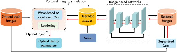
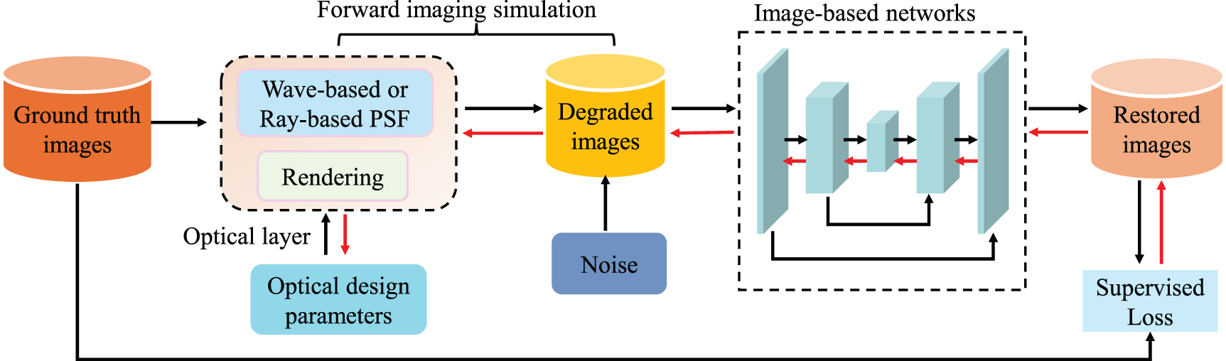
3.2.1. Data flow and network training

E2E optical design networks integrate optical image formation and image processing within a unified, differentiable learning framework. The learning objective is to jointly optimize the optical parameters, such as lens prescriptions or surface phase profiles, and the digital processing modules, including image restoration or task-specific networks, as explained in section 3.3.3 Figure 5 provides a schematic overview of this data flow, showing how both modules are connected by learnable components and optimized simultaneously.

Figure 5 Overview of E2E learning frameworks for optical design. The forward imaging simulation module models image degradations and provides differentiable links between optical parameters (e.g. lens prescriptions or surface phase profiles) and image-based training objectives, enabling joint optimization of optics and networks.

Download figure:

Standard image High-resolution image

To enable this joint training, the optical system is first modeled as a differentiable optical layer in the learning pipeline. Depending on the application, it includes wave-based propagation simulation for nano/micro-optical systems, or spatially varying ray tracing and its corresponding PSF convolution for multi-element lenses, as detailed in section 3.2.2.

The image-based networks are typically trained using paired data consisting of restored output images and high-quality GT targets. After training, the networks can be used to restore captured measurements from as-assembled optical systems. The most widely used loss function in E2E frameworks is the pixel-wise L2 loss, defined as:

Here denotes the reconstructed image, is the GT image, is the optical forward layer parameterized by , and Θ represents the network parameters to be optimized. This joint optimization framework enables the co-design of optics and downstream processing, distributing the burden of aberration correction across opto-mechanical elements and computational modules.

While pixel-wise L2 loss remains the most common choice in E2E networks, it often fails to capture perceptual or task-specific fidelity. To address this, perceptual losses computed from intermediate features of pretrained networks are introduced in tasks such as super-resolution and fluorescence localization microscopy [108], enabling better preservation of fine textures. In biomedical and edge-aware applications, SSIM loss and image gradient loss are added to enforce spatial consistency and boundary sharpness [112]. For semantic tasks like classification or depth estimation, cross-entropy, smooth L1, and intersection-over-union losses are commonly applied, as demonstrated in depth-guided detection [109] and time-of-flight pixel correction [110]. Adversarial loss components are also used in privacy-preserving systems to balance visual fidelity and feature suppression [113]. These tailored loss functions guide network training towards task-specific goals beyond mere pixel-level similarity.

3.2.2. Forward imaging simulation

In E2E optical design, the optical layer plays a central role by simulating the forward imaging process. This simulation serves to generate degraded images from ideal scene inputs and enables gradients to propagate through the optical module during training. Since collecting large quantities of real data from assembled optical systems is often labor-intensive and prone to misalignment, synthetic image generation is widely adopted. It offers high controllability, consistent pairing with GT data, and scalable data production. Two principal strategies are used to generate synthetic degraded images: rendering-based modeling and Fourier optics-based convolution.

Rendering-based methods simulate the physical propagation of rays from a 3D scene through the optical system, calculating their interactions with each surface along the optical path. This approach stems from rendering techniques in computer graphics [114], and has been adapted to model complex optical paths including reflection, refraction, and vignetting. In differentiable optical design, rendering involves per-pixel ray sampling, ray-surface intersection via iterative solvers [69], and evaluation of sensor response. It is computationally intensive due to high ray count and memory overhead during automatic differentiation. For example, simulating a wide field-of-view system with pixels and 64 rays per pixel requires more than one billion rays per frame. To improve efficiency, adjoint methods have been introduced to reduce memory consumption and accelerate gradient computation [68].

Fourier optics-based methods model optical degradation as a convolution between the GT image and the system’s PSF [115]. This approach is computationally efficient, fully differentiable, and widely adopted in learning-based optical design. Compared to rendering-based methods, it requires significantly fewer rays. For example, in a rotationally symmetric system, computing PSFs for only three fields with rays per pupil per field results in fewer than 15 000 rays in total, enabling rapid data generation during training.

When the PSF is shift-invariant, the degraded image is given by:

where denotes convolution and η denotes statistical noise. The degraded image depends on the wavelength λ and the object distance d.

For realistic optical systems with field-dependent aberrations, shift-variant PSFs are required. In such cases, the image is synthesized by summing locally convolved image patches:

where are spatial masks that localize each PSF to its corresponding image region, and i indexes the sampled fields with a field number N, i.e. N = 9. To accelerate the convolution process, computations are typically performed in the Fourier domain using FFT. Note that high-fidelity image synthesis may require higher-dimensional PSF models, such as 3D PSF for spatially varying scenes [100] and 4D PSF for depth-aware imaging [103].

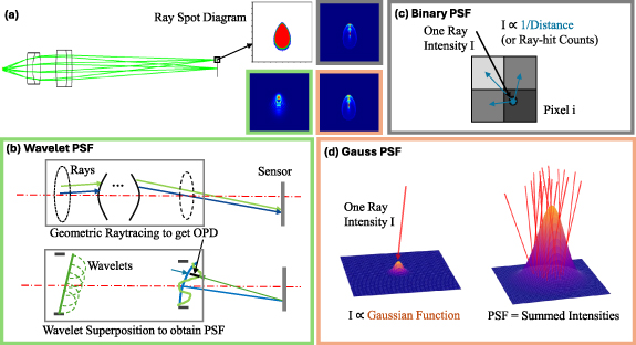
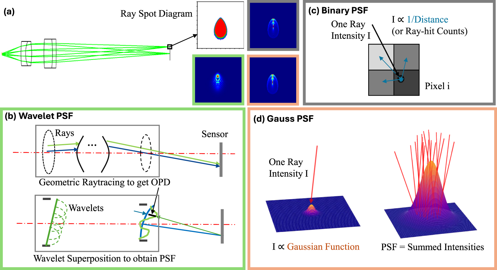
PSFs can be obtained either through experimental measurements or simulations. Simulation-based PSFs fall into two main types [39]: ray-based and wave-based. Ray-based methods, typically implemented via DRT (see section 2.2.2), model geometric aberrations and are often shift-invariant. Common implementations include binary ray counting (‘Binary PSF’) [111] and Gaussian-weighted energy aggregation (‘Gauss PSF’) [66, 101, 102, 116]. Wave-based PSFs can be computed via superposing wavelets arriving at the exit pupil (‘Wavelet PSF’) in geometric optical designs [100, 117, 118], or directly compute from simplified propagation models in DOE or metalens designs [44, 109], detailed in section 3.2.3. As shown in figure 6, the wavelet PSF exhibits clear diffraction features even in low-NA, low magnification microscopy systems, whereas the other two PSFs preserve only the coarse geometric shape. These differences can significantly affect the performance of learning-based image reconstruction.

Figure 6 Comparison of three PSF simulation models for a low-NA microscopy system, highlighting the distinct diffraction features captured by the Wavelet PSF. (a) Spot diagram generated by geometric ray tracing. (b) Wavelet PSF is computed by coherently superposing wavelets at the exit pupil, with phase delays obtained from the optical path difference (OPD) in ray tracing. (c) Binary PSF estimates intensity by assigning 0–1 portions to ray-pixel intersections based on distances to adjacent pixel centers. (d) Gauss PSF models each ray as a Gaussian function centered at its intersection point.

Download figure:

Standard image High-resolution image

In experimental settings, the fidelity of the measured PSF is influenced by sampling frequency, sensor noise and the optical performance of the measurement setup. Insufficient spatial sampling may suppress high-frequency aberration signatures or introduce aliasing [115]; photon and read noise propagate directly into the recorded PSF [119]; and the MTF of measurement optics can distort the measured response relative to the true system PSF [120]. These effects are particularly pronounced in high-resolution microscopy [95, 119], where systems operate near the diffraction limit and are highly sensitive to defocus and element misalignment.

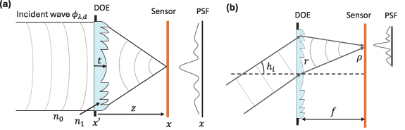
3.2.3. Wave-based propagation

Wave-based PSF modeling offers a physically accurate description of image formation in optical systems where diffraction and interference play a dominant role. According to scalar wave optics [115], the phase of a monochromatic wavefront is delayed by the optical path length when passing through a material:

where λ is the wavelength, Δn represents the refractive index difference, and t is the local thickness of the optical element, as illustrated in figure 7(a). Then, the wavefront propagates to the sensor plane typically following Fresnel diffraction under the paraxial approximation, which is valid when . For a planar incoming wavefront, the PSF captured by the sensor is given by:

where A is the complex amplitude at the pupil, and C is a constant scaling factor. The depth-dependent phase term φd is included to model defocus effects when the object is at a finite distance d, a strategy commonly used in depth estimation DOE systems [109, 121]. This formulation typically results in a spatially invariant PSF that is constrained by paraxial approximation assumption, which neglects off-axis aberrations and is limited to narrow FOVs.

Figure 7 Differentiable wave-based PSF modeling for micro-optical imaging. (a) Shift-invariant PSF computed under the paraxial approximation for small FOV using Fresnel propagation. (b) Field-dependent PSF subscripted using h adapted for wide-angle imaging, where phase modulation varies with the incidence angle and radial position of off-axis wavefronts.

Download figure:

Standard image High-resolution image

To extend the model to wide-angle imaging, the phase modulation must incorporate field dependence. For an off-axis object point, as illustrated in figure 7(b), the incoming wavefront is tilted, and accurate focusing requires the phase term to explicitly depend on the incidence angle, radial position, and focal distance [99]. Designing DOE to optimally focus multiple off-axis fields leads to phase conflicts that cannot be resolved analytically. In such cases, an optimized phase profile is adopted, and corresponding field-dependent PS are evaluated numerically.

Several numerical methods are available to compute such wave-based PSFs. Fresnel diffraction remains the most used due to its computational simplicity and differentiability. The ASM [115] improves accuracy for larger propagation angles and non-paraxial cases, using the plane-wave decomposition. For subwavelength features or highly scattering structures, full-wave solvers [63] such as FDTD or FEM provide rigorous modeling by directly solving Maxwell’s equations. However, due to their computational cost, such methods are rarely used in E2E learning. Instead, Fresnel diffraction and ASM remain the dominant approaches, offering a practical balance between physical fidelity and numerical efficiency.

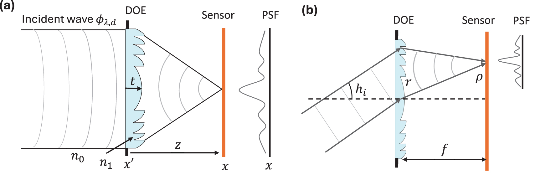
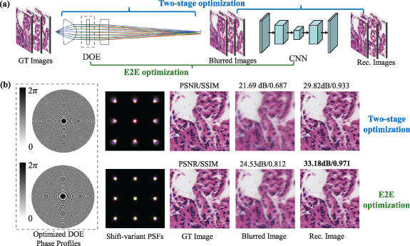
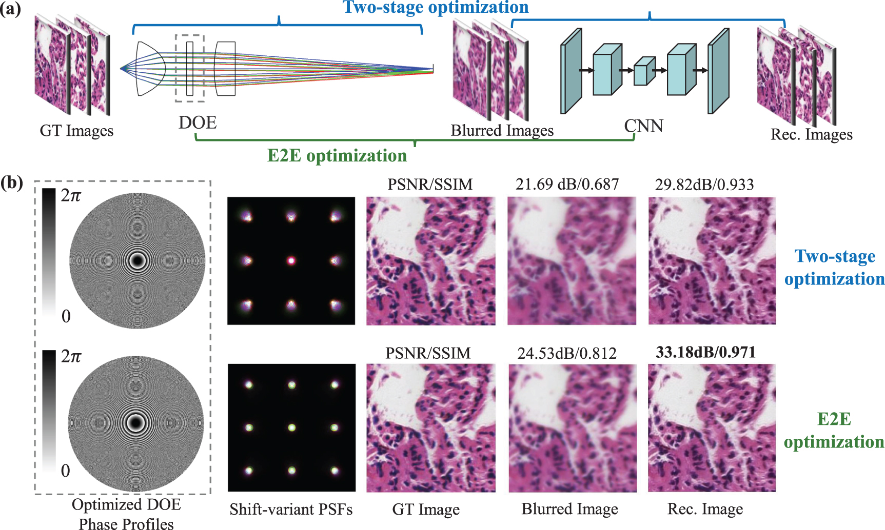
3.2.4. E2E network design example on an achromatic DOE

To illustrate the practical behavior of E2E co-optimization, we perform the co-design of a DOE for a compact achromatic microscope, as seen in figure 8(a). This example extends our previous work [39], where a miniature monochromatic microscope with two aspheric singlet lenses was designed. We further introduce a rotationally symmetric DOE to correct chromatic aberrations, while keeping the optical parameters, network architecture and noise settings unchanged.

Figure 8 E2E design example for a compact achromatic microscope optimized with CNN reconstruction. (a) Illustration of the two-stage and E2E optimization framework.(b) Optimized DOE phase profiles, corresponding shift-variant PSFs, and example reconstructed (Rec.) images for the two-stage and E2E optimization strategies.

Download figure:

Standard image High-resolution image

To enable the network training, a set of GT images is propagated through the parameterized DOE represented by Zernike coefficients and two lenses to generate synthetic blurred images using equation (5), which are subsequently restored by a CNN. The DOE phase profile and network weights are jointly optimized through image-domain loss in equation (3). This approach differs from the two-stage workflow, where the optical system is first optimized using a multi-wavelength spot-size merit function and the resulting images are then processed by the deblurring CNN network. Figure 8(b) shows the optimized DOE phase profiles, the corresponding shift-variant PSFs, and reconstructed images for both strategies. In the two-stage approach, the DOE primarily reduces the mean spot size of three selective wavelengths, whereas the E2E method adapts the DOE to improve the image-domain reconstruction quality. Quantitatively, E2E optimization yields an increase of approximately 3.36 dB in PSNR and an improvement of about 4% in SSIM, demonstrating that joint optimization can provide higher imaging quality than optimizing the optics and the network separately.

To outline the current landscape of learning-based E2E optical design, we reviewed and compared 24 representative methods from recent literature. These approaches span conventional refractive lenses, freeform elements, diffractive optics, and meta-optics, and are applied to a variety of imaging tasks including depth estimation, super-resolution microscopy and HSI, as summarized in table 3. Building on this overview, table 4 presents 6 selected design examples with explicit system specifications and reported performance gains, illustrating how E2E co-optimization can improve both optical performance and image reconstruction quality.

Table 3. Summary of representative end-to-end optical design methods, including optical element types and parameters, forward imaging models, network architectures, and application domains.

AuthorYearOptical componentsOptical parametersImaging modelsNetworkApplicationsElmalcm et al [97]2018single DOEradial profile heightsCNNEDOFChang and Wetzstein [109]2019single lensZernike coefficientsU-Netdepth sensingWu et al [121]2019single DOEheight mapU-Netdepth sensingSun et al [122]2020single DOEradial profile heightsCNNHDRSun et al [123]2020single DOEPSFCNNsuper-resolutionDun et al [98]2020single DOEradial profile heightsRes-UNetHSINehme et al [108]2020single DOEheight mapRes-UNetlocalization microscopyTseng et al [118]2021compound lensesthickness, surface radius, aspheric coefficientsU-Netautomotive object detection, Low light imagingSun et al [69]2021compound lensessurface radius, aspheric coefficientsRenderingGANLFOV, EDOFLi et al [102]2021single lensaspheric coefficientsRes-UNetLFOVBaek et al [124]2021single DOEphase profileU-Nethyperspectral-depth ImagingIkoma et al [125]2021single DOEradial profile heightsU-Netdepth sensingBurgos et al [126]2021single metalensphase profileCNNoptical neural networksTseng et al [43]2021single metalensphase profileU-NetLFOVHinojosa et al [127]2021single DOEZernike coefficientsCNNhuman pose estimationArguello et al [128]2021single DOEheight mapU-Netsnapshot HSIWang et al [68]2022compound lensessurface radius and aspheric coefficientsRenderingU-NetLFOV, EDOFShi et al [129]2022single DOEheight mapU-Netoptical cloakingLi et al [130]2022single DOEheight mapRes-UNetsnapshot HSIZhang et al [112]2022single DOEPSFRNNsuper-resolutionYang et al [116]2023off-axis mirrorsfreeform surface coefficientsRes-UNetfreeform imagingCôté et al [66]2023compound lensesthickness, surface radius, and glass variablesRetinaNetobject detectionZhang et al [131]2023single metalensphase profileU-Netsnapshot HSIYang et al [132]2024compound lensesthickness, surface radius and aspheric coefficientsU-NetEDOF

Table 4. E2E design examples illustrate optical optimization and image reconstruction performance across practical DOE, metasurface, aspheric and freeform imaging systems.

Designed optical systemsComments on network prediction performanceSingle DOE for snapshot HSI [98] EFL:50 mm, aperture: 8 mm (2