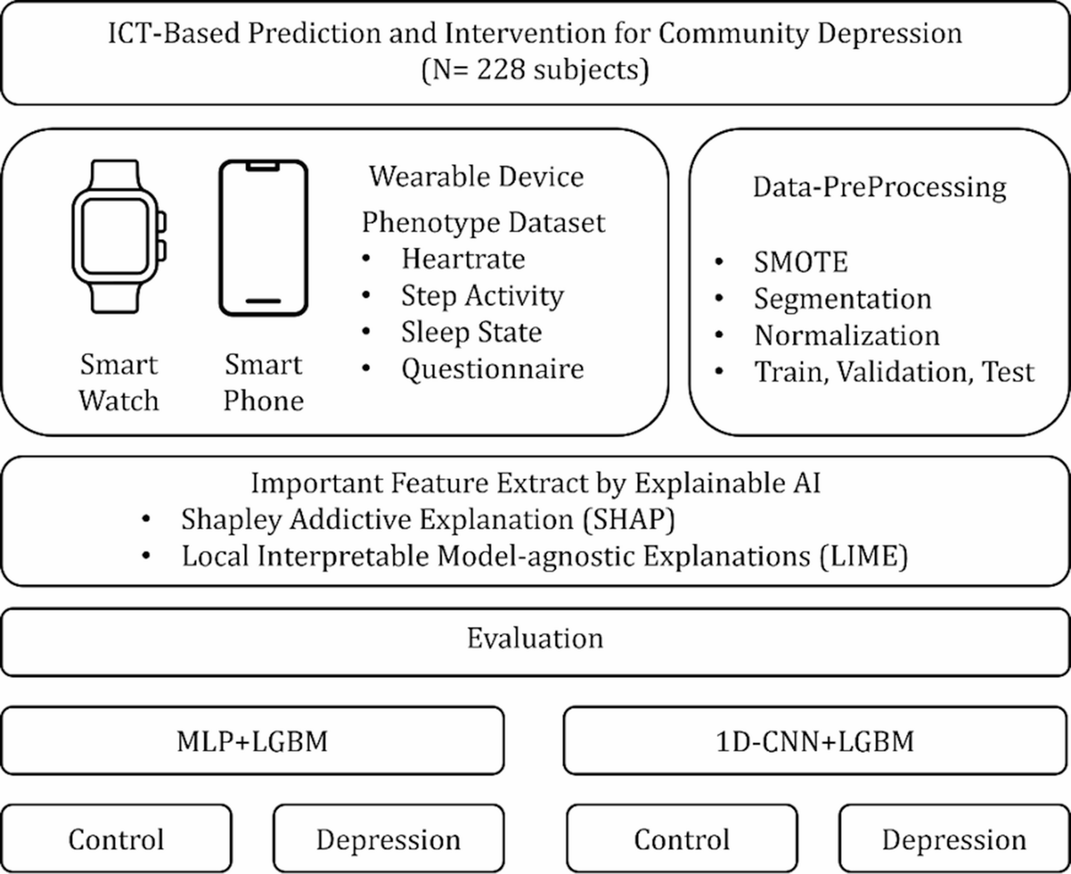
SHAP (SHapley Additive eXplanations) is one of the representative XAI techniques used to interpret the prediction results of machine learning models. It has the advantage of quantifying and visualizing how much and in which direction each feature contributes to the model’s prediction outcome. The SHAP value, obtained through this method, serves as a key component in decomposing the prediction output, indicating the extent to which each feature influences the model’s overall prediction value, as described in Eq. (2).

$$f(x)=E\left(\left[f\left(x\right)\right]\right)+\sum_^n\phi_i$$

(2)

In this equation, f(x) represents the model’s prediction for an input sample x, and E[f(x)] denotes the average prediction across the entire dataset, serving as the baseline value. ϕi refers to the contribution of feature i to the model’s prediction, and by comparing these contributions, the relative importance of each feature to the final prediction can be systematically accessed. Therefore, SHAP values enable the decomposition of complex decision-making processes within the model, allowing the identification of which features exert a stronger or weaker influence on the output prediction. Based on this interpretability, this study employed SHAP-based visualization techniques, namely the beeswarm plot and waterfall plot, to analyze the key features involved in the depression prediction models. The beeswarm plot summarizes SHAP values across all samples, allowing for an overall assessment of feature importance and the direction of their effects, whereas the waterfall plot visualizes, for each individual sample, how features sequentially contribute to the deviation from the baseline prediction. The analysis results are presented in Figs. 4 and 5.

The SHAP beeswarm plot analysis demonstrated that ‘Night Sleep Time’ consistently emerged as the most influential variable in XGBoost and LightGBM models, whereas ‘Day Sleep Time’ was identified as the most significant predictor in the first model. The contribution of ‘Night Sleep Time’ to the prediction was particularly prominent near its median range, as indicated by the dense concentration of SHAP values around the central axis. This observation suggests that maintaining a moderate duration of night sleep may be associated with a reduced risk of depression. Additional features such as ‘Age’, ‘Day Sleep Time’, ‘Religion Activity’, ‘Income Responsibility’, and ‘Diabetes’ were repeatedly highlighted as key predictors across all three models. A reduction in ‘Night Sleep Time’ generally corresponded to an increased likelihood of depressive outcomes, as inferred from the directionality of SHAP values. Conversely, active engagement in social behaviors, including participation in community or social groups such as ‘Social Club’ activities, appeared to mitigate predicted depression risks, underscoring the potential psychological benefits of social connectedness. The convergence of feature importance across ensemble models reinforces the interpretability and consistency of these predictors in relation to depressive symptomatology derived from behavioral and demographic input variables.

The waterfall plot analysis provided additional validation of feature contributions at the individual level. In all three models, ‘Night Sleep Time’ consistently exerted the strongest negative impact on the model output, significantly lowering the predicted probability of depression. This reinforces its role as a protective factor, suggesting that maintaining sufficient night sleep duration may help mitigate depressive risk. Other features such as ‘ReligionActivity’, ‘IncomeResponsibility’, and ‘Night Deep Time’ also contributed to reduced prediction scores, indicating their potential positive influence on mental health. In contrast, variables including Step activity, Diabetes, and Stroke were associated with an upward shift in the prediction score, implying that lower physical activity and the presence of chronic medical conditions may increase the likelihood of depression. These results emphasize the consistent explanatory strength of sleep related features, along with behavioral and clinical indicators, in shaping individualized depression risk estimations across multiple models.

SHAP beeswarm plots for depression prediction models: (A) Random Forest, (B) XGBoost, and (C) LightGBM. Each plot shows the global feature importance and the direction of influence of features on the model’s prediction. Colors indicate the original feature values, and features are sorted by their mean absolute SHAP values

SHAP waterfall plots show the contribution of each feature to the final prediction for a representative individual. (a) Random Forest, (b) XGBoost, and (c) LightGBM. Each plot illustrates how the model’s prediction is built from the base value by adding the SHAP values of individual features. Features pushing the prediction higher are shown in red, while those lowering it are shown in blue

LIME (Local Interpretable Model-agnostic Explanations) is a representative XAI technique designed to provide local interpretability of machine learning model predictions. For a complex and nonlinear model f, LIME approximates the prediction for a specific input sample x using a simpler, interpretable model g. This objective can be expressed as follows in Eq. (3) where L(f, g,πx) represents the loss function that measures the discrepancy between the predictions of the original model f and the interpretable model g under a locality distribution πx​ around the sample x, and Ω(g) denotes a penalty term for the complexity of the surrogate model g.

$$\underset\mathcal L(f,g,_)+\Omega(g)$$

(3)

Through this optimization process, LIME constructs a simple linear model or decision tree that explains the major features contributing to the specific prediction outcome. In this study, LIME was used in parallel with SHAP, with particular attention given to LIME’s ability to provide local explanations. By training a simple model centered around each sample, LIME enables the intuitive identification of key features that most significantly influenced each prediction. This approach allowed us to examine the differences in feature contributions between individuals predicted as depressed and those classified as controls, thereby enhancing the interpretability and trustworthiness of predictions made by the complex model.

Based on the LIME analysis results presented in Fig. 6, we further examined the key features that influenced prediction outcomes at the individual level. Among the participants classified as control, features such as ‘Night Sleep Time’, ‘Total Sleep Time’, and ‘HR Min’ were consistently associated with predictions toward the non-depressive class. Particularly, individuals with sufficient night and total sleep durations showed markedly lower predicted probabilities of depression, aligning with trends identified in the global SHAP analysis. In contrast, for individuals with higher predicted probabilities of depression, features such as ‘Welfare_BasicLiving’, ‘Stroke’, ‘Diabetes’, and ‘Barrier_NoTime’ contributed positively to the model output. Moreover, additional indicators including ‘Support for Adult Children’ and ‘Welfare_Disability’ appeared as influential factors in the third case, reflecting socioeconomic and caregiving related stressors. These findings suggest that while sleep-related features serve as protective factors at the individual level, the presence of chronic illness, limited time resources, and socioeconomic burden emerge as key drivers that elevate the predicted risk of depression.

Local explanations of depression prediction using LIME across three ensemble models: (A) Random Forest, (B) XGBoost, and (C) LightGBM. Each plot illustrates the feature contributions for a selected individual, with bars representing the extent to which each feature increased or decreased the predicted probability of depression. The visualizations highlight how specific features locally influenced the model’s decision for each sample

To evaluate the contribution of individual features to model predictions, feature importance analysis was performed using both SHAP and LIME methods. Based on the resulting importance scores, top-ranked features were selected for subsequent model training. To further assess potential redundancy among the selected features, a correlation matrix analysis was conducted on the integrated feature set, as shown in Fig. 7. The analysis revealed that most feature pairs exhibited low correlation coefficients, with the maximum absolute correlation observed at approximately 0.77. These results suggest that the selected features primarily provide independent information, thereby supporting the robustness of the subsequent deep learning model training based on the selected feature sets.

Correlation matrix of the unified top features selected from Random Forest, XGBoost, and LightGBM models

Through the preceding analysis, key features were extracted from the three ensemble models previously described Random Forest, XGBoost, LightGBM. In this study, the top 15 important features identified from each model were selected to systematically evaluate the impact of feature selection on the performance of hybrid deep learning models. The hybrid models employed for evaluation were the 1D-CNN and MLP, each integrated with LightGBM, as previously outlined. Two experimental conditions were compared by training models either with the full set of features or exclusively with the selected important features. Model performance was evaluated using standard classification metrics, namely accuracy, precision, recall, F1-score, and area under the ROC curve (AUC), as defined by Eqs. (4), (5), (6), (7), and (8) respectively.

$$F1-score=2\times\frac$$

(7)

$$AUC=\int_0^1TPR(x)\;dx$$

(8)

The predictive performance of each model was first assessed using confusion matrices, with results for the 1D-CNN+LightGBM model shown in Fig. 8 and for the MLP + LightGBM model in Fig. 9. In addition, ROC curves and AUC scores were analyzed during 5-Fold cross validation to evaluate the variability and generalization performance of the models, as shown in Figs. 10 and 11. A comprehensive summary of the quantitative results for all experimental conditions was provided Table 6, enabling an integrated comparison of the model’s classification performance. The experimental results confirmed that models trained using selected important features consistently outperformed those trained with all available features. Particularly, MLP + LightGBM hybrid model, trained with features selected via XGBoost, achieved the highest classification accuracy 93.43%. These findings empirically demonstrate that effective feature selection can significantly enhance model predictive performance, while simultaneously improving learning efficiency and model interpretability.

Confusion matrices for the 1D-CNN + LightGBM model: (A) using all features, (B) using features selected by Random Forest, (C) using features selected by XGBoost, and (D) using features selected by LightGBM

Confusion matrices for the MLP + LightGBM model: (A) using all features, (B) using features selected by Random Forest, (C) using features selected by XGBoost, and (D) using features selected by LightGBM

ROC curves for the 1D-CNN + LightGBM model: (A) using all features, (B) using features selected by Random Forest, (C) using features selected by XGBoost, and (D) using features selected by LightGBM

ROC curves for the MLP + LightGBM model: (A) using all features, (B) using features selected by Random Forest, (C) using features selected by XGBoost, and (D) using features selected by LightGBM