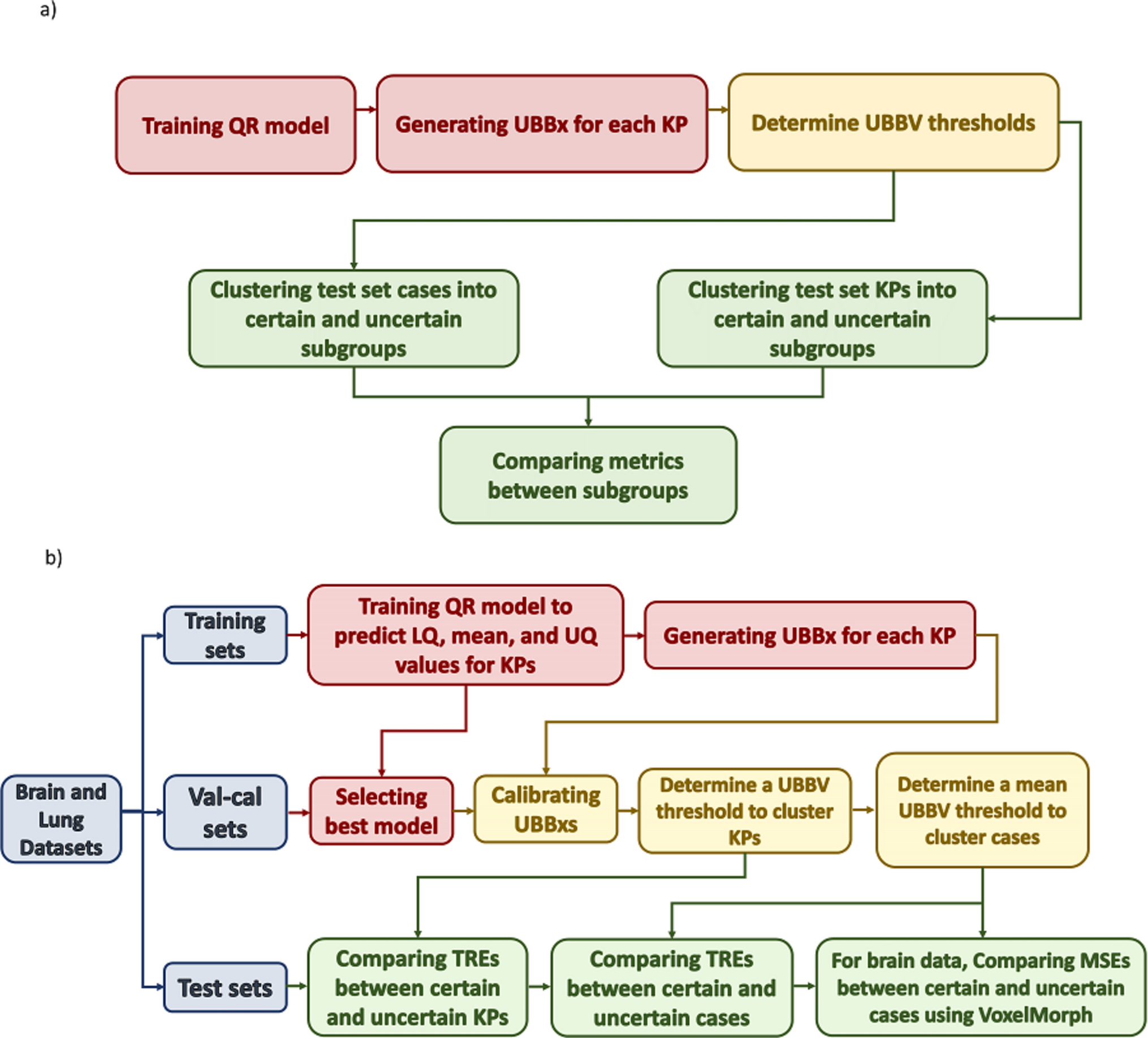
The proposed methodology involves several stages. First, a DL-based registration model is trained using QR to concurrently predict a dense displacement field (DDF) for alignment and its corresponding uncertainty bounds. Subsequently, CP is applied to these bounds to ensure the statistical reliability of the final uncertainty estimates. This process yields uncertainty bounding boxes (UBBxs), which represent uncertainty around each predicted keypoint (KP). From these, the uncertainty bounding box volume (UBBV) is computed as a quantitative measure reflecting the spatial extent of uncertainty for each KP. These UBBVs are then used to cluster the registered test set cases into “certain” and “uncertain” subgroups based on their quantified levels of uncertainty. Finally, the efficacy of the UQ is validated through multiple quantitative procedures. Figure 1 illustrates a summary of the study design.

Fig. 1

The flowchart illustrates the CONReg pipeline. The QR model was trained to generate UBBx for each KP. The best model was selected, and UBBx was calibrated on the validation-calibration sets. KPs were classified into certain and uncertain subgroups based on UBBV using Gaussian mixture model (GMM). Additionally, cases were classified into certain and uncertain subgroups based on the mean UBBV of KPs using GMM. The mean target registration error (TRE) was evaluated in the KP and case subgroups in the test sets. Furthermore, we used a valid registration model, VoxelMorph, to register brain images within the subgroups and compared the mean squared errors (MSEs)

Datasets

In this study, we used three different databases, which include brain MRI and lung CT datasets from several challenges:

OASIS

This study utilized 414 3D whole-brain MR scans from the Open Access Series of Imaging Studies [25, 26], provided through the Learn2Reg 2021 Challenge. The dataset features a cross-sectional study of participants who were either healthy or diagnosed with Alzheimer’s disease. Cases were accompanied by ground truth segmentation masks for specific regions of interest. For the registration tasks, random cases were paired, with each image serving as both a fixed and moving image across different pairings.

BraTS-Reg

The BraTS-Reg 2022 Challenge dataset consists of 140 pairs of pre-operative and post-operative brain MR images from patients with diffuse glioma [27]. For registration, the pre-operative scan was designated as the fixed image, while the post-operative scan was used as the moving image.

NLST

The Learn2Reg 2023 Challenge provided the NLST dataset, which consisted of 219 pairs of chest CT scans [28,29,30]. Each pair included a baseline and a follow-up scan, which were assigned as the fixed and moving images, respectively.

All datasets were partitioned into training (70%), validation-calibration (10%), and test (20%) sets at the patient level. Before training, all input images were resized to a uniform dimension, with the OASIS and BraTS-Reg datasets resized to 128 × 128 × 128 voxels and the NLST dataset resized to 96 × 96 × 96 voxels. Also, each image was independently normalized, using all nonzero voxels to compute the minimum and maximum voxel values.

Model DevelopmentKeypoint Generation

Anatomically defined KPs are a critical component of this methodology, as they provide specific locations for calculating the TRE and Pinball loss functions. These losses are essential for training the model to predict both accurate alignments and reliable uncertainty bounds. For a given keypoint \(i\), TRE is defined as the Euclidean distance between the predicted and ground-truth positions:

$$_}=\sqrt_}^}-_}^}\right.\right)}^+_}^}-_}^}\right.\right)}^+_}^}-_}^}\right.\right)}^}$$

where \(_}^}, _}^}, _}^}\) denote the predicted coordinates of the \(i\) th keypoint, and \(_}^}, _}^}, _}^}\) denote the corresponding ground-truth coordinates. Since the OASIS and BraTS-Reg datasets lacked pre-defined KPs for this purpose, we employed BrainMorph [31], a subtype of KeyMorph framework [32], designed for robust brain MRI registration. BrainMorph automatically generated 512 corresponding KPs for each pair of fixed and moving images. This process ensured that a consistent set of KPs was available to guide the model’s training. This automated generation was not required for the NLST dataset, which already provided pre-defined KPs.

Overview of Conformalized Quantile Regression

Our methodology is centered on CQR, a statistical framework that generates prediction intervals with formal coverage guarantees by integrating QR with the principles of CP. CP provides a model-agnostic method for UQ. For a dataset of exchangeable pairs \((_}, _})\), where each Xᵢ represents an input feature and Yᵢ its associated outcome, the objective is to construct a prediction set \(C(_+1})\) for a new instance \(_+1}\) that satisfies the marginal coverage guarantee:

$$P(_+1}\in C(_+1}))\ge 1- a$$

where \(1-a\) is the user-specified confidence level. CQR enhances CP by incorporating quantile regression, enabling it to more effectively handle heteroscedasticity. The process begins by using a model trained with QR to predict an initial interval:

$$\left[}_(X),}_(X)\right]$$

where \(}_}\left(X\right)\) is estimated conditional \(a\)-quantile of the response given input \(X\), and \(a\) is the error rate. This interval is then calibrated using a dedicated calibration set. For each calibration sample \((_}, _})\), a nonconformity score is calculated to measure the distance the true value falls outside the predicted interval:

$$_=max\left\}_\left(_\right)-_,_-}_\left(_\right)\right\}$$

where \(_}\) is the observed outcome for calibration input \(_}\). A calibration term \(Q\) is then determined as the \(1-a\) quantile of these empirical scores. This term adjusts the initial interval to form the final, calibrated prediction set for a new input \(_+1}\):

$$C\left(_\right)=\left[}_\left(_\right)-Q,}_\left(_\right)+Q\right]$$

In our work, we applied this CQR methodology sequentially. We first trained our DL-based registration model using QR to generate the initial uncertainty bounds for DDF. Subsequently, we employed the conformalization step to calibrate these bounds, resulting in statistically valid uncertainty estimates. The specific implementations of the model training and the calibration procedure are detailed in the following sections.

Model Training

We employed a 3D U-Net architecture to predict DDF from paired fixed and moving images. A DDF represents the vector field required to map each voxel from the moving image to its corresponding location in the fixed image. To quantify registration uncertainty, we adapt this architecture using QR. Instead of predicting a single displacement vector for each voxel, our model is trained to estimate three distinct DDFs corresponding to a lower quantile (LowQ), a mean, and an upper quantile (UpQ) of the displacement distribution. This approach yields a predictive interval for the displacement of each voxel, directly representing the model’s spatial uncertainty. Details of the network specification are provided in Table 1.

Table 1 Architecture details of the proposed quantile-based U-Net used for image registration

For a given quantile τ, the DDF is represented as the displacement vector for each voxel at position \((x,y,z)\). The DDF at quantile τ is expressed as

$$DD_(x,y,z)=\left[\begin\Delta }_\\ \Delta }_\\ \Delta }_\end\right]$$

where \(\Delta _\), \(\Delta _\), \(\Delta _\) represent the displacement of the voxel at position \((x,y,z)\) along the x, y, and z dimensions, respectively, for \(\tau \epsilon \\). Therefore, for a given voxel, the displacement along dimension \(j\) (\(j \in \\)) across LowQ, mean, and UpQ is represented as

$$_}(x,y,z)=\left[\begin_}\\ _}_}}\\ _}\end\right]$$

where \(_}\), \(_}\), and \(_}\), represent the displacement for the dimension \(j\) at the LowQ, mean, and UpQ, respectively. The moving image and its segmentation mask (if available) were warped using the mean DDF to generate the registered image and mask, respectively. Additionally, the KPs in the moving image were warped using LowQ, mean, and UpQ DDFs.

To train the model, a combined loss function was used, incorporating Dice and MSE losses for image registration, and pinball and TRE losses for KP displacement. The pinball loss is applied to the displacement errors of the KPs, comparing their predicted positions (\(}_}\)) with their true positions (\(_}\)). For a spatial dimension \(j\) and a target quantile \(\tau\), the Pinball loss is calculated as follows:

$$_\left(_},}_}\right)=\left\\tau \left(_}-}_}\right),\hspace\hspace\hspace\hspace \, }} \, _}\ge }_}\\ (1-\tau )\left(}_}-_}\right),\hspace\hspace\hspace\hspace \, }} \, _}<}_}\end\right.$$

The total pinball loss aggregates errors across all dimensions \(j\) and quantiles:

$$\text=\sum_} \sum_,UpQ\}} _\left(_},}_}\right)$$

The total loss function is the weighted sum of Dice loss, MSE loss, Pinball loss, and TRE loss:

$$Total\ loss=a\ KPs\ pinball\ loss+B\ mean\ KPs\ TRE\ loss+\ \gamma\ \text+\ \delta\ \text$$

where \(\alpha , \beta ,\gamma , and \delta\) are scaling factors that balance the loss components, ensuring that both the image alignment and KP displacement are optimized during training. Where \(\alpha , \beta ,\gamma , and \delta\) are scaling factors that balance the loss components, ensuring that both the image alignment and KP displacement are optimized during training. The weights were empirically tuned for each dataset based on performance on their respective validation-calibration sets to balance registration accuracy and uncertainty quantification. The final values used are provided in Online Resource 1.

Within this training framework, the LowQ and UpQ DDFs are predicted densely across the image but are supervised only at KP locations using the Pinball loss. Because the quantile heads share a common encoder–decoder backbone with the mean DDF branch, the dense spatial losses (MSE and Dice) applied to the mean branch propagate spatial consistency and anatomical smoothness to the quantile fields. This shared-backbone design ensures that even with sparse supervision at KPs, the quantile DDFs maintain coherent voxelwise structure across the entire volume.

We optimized the models using the Adam optimizer with a learning rate of 1e-4 and applied a cosine annealing learning rate scheduler over a maximum of 200 epochs. Additionally, a dropout rate of 20% was also utilized to prevent overfitting. The best model was selected according to the lowest mean KP TRE on the validation-calibration set. Specifically, after each training epoch, the model was evaluated on this set, and the mean Euclidean distance between the predicted and ground-truth KP positions was computed. The model with the lowest mean TRE was retained as the best model for subsequent testing, ensuring optimal registration accuracy on unseen data.

Conformalized Quantile Regression

To incorporate statistical guarantees into the registration process, we applied CP to conformalize the QR model after training. Specifically, CP was employed as a post hoc calibration step that adjusts the predictive intervals produced by the QR model to achieve the desired nominal coverage, without altering the underlying network or retraining.

As described in the previous section, the base model predicts the LowQ and UpQ for the final position of KPs in the registered image for each dimension. In this section, we use CP to adjust these bounds and validate them statistically. This is implemented by calculating nonconformity scores in the validation-calibration sets, which are then used to determine a nonconformity threshold. When the model is evaluated on the test sets, the LowQ and UpQ predicted by the model for the x, y, and z values of each KP are refined by applying the thresholds. This results in the generation of an UBBx for each KP using the adjusted values.

Nonconformity scores were computed on validation-calibration sets by measuring the maximum deviation between the true KP displacements and the predicted LowQ and UpQ bounds. Specifically, for each KP \(i\) and dimension \(j\), the nonconformity score was defined as

$$_}=max\left(\left|_,\text}-}_,\text}^}\right|,\left|_,\text}-}_,\text}^}\right|\right)$$

where \(_,\text}\) is the true position of KP \(i\) in dimension \(j\), \(}_,\text}}^}\) and \(}_,\text}}^}\) are the predicted LowQ and UpQ bounds for KP \(i\) in dimension \(j\). These scores were calculated separately for each dimension and aggregated across the validation-calibration samples. A threshold of these nonconformity scores for each dimension was then determined at a significance level of

$$\alpha = 1 - (UpQ - LowQ)$$

On the test set, the predicted quantile bounds were adjusted using this threshold for each KP \(i\) and dimension \(j\) and threshold \(_}\) (determined from the calibration step). Adjusted predicted quantile bounds are as follows:

$$\left[}_,\text}^}-_},}_,\text}^}+_}\right]$$

This process generates a 3D UBBx for each KP. The coverage probability is calculated as the proportion of KPs whose true positions fall within their predicted UBBxs. In this context, this is specifically defined as the proportion of KPs whose true positions in all three dimensions fall within the adjusted LowQ and UpQ bounds. The coverage probability is computed as

$$\text=\frac\sum_^ \prod_} }\left(_,\text}\in \left[_,\text}^}-_},_,\text}^}+_}\right]\right)$$

where N denotes the total number of test set KPs, \(_,\text}\) is the true position of KP \(i\) in dimension \(j\), \(}_,\text}}^}\) and \(}_,\text}}^}\) are the predicted LowQ and UpQ bounds for KP \(i\) in dimension \(j\), and \(_}\) is the adjusting quantile value derived from CP. Figure 2 shows the possible positions of the KPs based on the UBBx.

Fig. 2

Possible positions of the KPs based on the UBBx: Two scenarios are illustrated: A KP within the UBBx and B KP outside the UBBx. Coverage is defined as the proportion of KPs in scenario A relative to the total number of KPs. CLQ, conformalized lower quantile; CUQ, conformalized upper quantile; LM, landmark

Selecting Appropriate UpQ and LowQ

The selection of appropriate UpQ and LowQ depends on the target CI and the number of image dimensions (2D or 3D). As the LowQ and UpQ are determined independently for each dimension, the confidence level is adjusted to achieve a joint CI across all dimensions for the UBBx. The adjusted significance level (α) is calculated as

$$1-\sqrt[\text\text].\text95\text\right)}$$

And the UpQ and LowQ for each dimension are then defined as

$$\beginUpQ=1-\frac\text].\text95\text\right)}}& LowQ=\frac\text].\text95\text)}}\end$$

In this study, we targeted a 95% CI, corresponding to a 95% probability that a KP lies within the UBBx across all three dimensions. Using the above formulas for three dimensions and a CI of 0.95, the \(a\), UpQ, and LowQ for each dimension were set to 0.0170, 0.9915, and 0.0085, respectively, to ensure a 95% joint coverage probability for the UBBx.

Quantifying Uncertainty and Stratifying Outcomes

The CQR process yields a calibrated 3D UBBx for each KP. To translate this geometric output into a practical metric, we quantify the uncertainty at the KP level by its UBBV. A larger volume intuitively corresponds to greater uncertainty in the predicted location of the KP. To assess the overall uncertainty for an entire registered case, we compute the mean UBBV across all KPs within that case.

These quantitative metrics serve as the basis for stratifying registration outcomes. We apply a GMM to the UBBVs (for KPs) and the mean UBBVs (for cases) within the validation-calibration set to establish data-driven thresholds. These thresholds are then used to classify KPs and entire cases in the test set into two distinct subgroups: “certain” (KPs and cases where their UBBV is below the UBBV threshold) or “uncertain” (KPs and cases where their UBBV exceeds the UBBV threshold). This stratification provides a practical tool for automated quality control. Additional methodological notes are provided in Online Resource 2. The subsequent section describes the validation experiments performed to confirm that these uncertainty metrics and classifications are strongly correlated with registration accuracy.

Model Validation

To validate the proposed framework, we performed a series of quantitative experiments on the test sets:

Correlation Analysis

We statistically analyzed the correlation between our uncertainty metrics and TRE. This was performed at both the KP level (UBBV vs. TRE) and the case level (mean UBBV vs. mean TRE).

Subgroup Comparison

We assessed the efficacy of our stratification by statistically comparing the TRE between the certain and uncertain subgroups for both KPs and cases. For the OASIS dataset, we additionally compared the Dice Similarity Coefficient (DSC), which is a measure of spatial overlap between the predicted and ground-truth regions of interest (ROIs), between the certain and uncertain subgroups.

External Validation (for Brain Datasets)

For brain datasets, we conducted an external validation by using a pretrained VoxelMorph model to register the cases from our classified subgroups. We then statistically compared the MSE of the resulting registrations between the certain and uncertain subgroups.

Statistical Analysis

The Kolmogorov–Smirnov test was employed to assess the normality of the data. Quantitative variables are presented as either the mean ± standard deviation or the median (interquartile range), depending on the distribution of the data. Comparisons between groups were performed using the t-test or the Mann–Whitney U test (based on data distribution). Correlations between variables were evaluated using the Pearson or Spearman rank correlation test, depending on the data distribution. All statistical analyses were conducted with SPSS 20 software, and a p-value of < 0.05 was considered statistically significant.