Data Acquisition

This study exploited PET/CT brain images of 219 patients presenting with head and neck malignant lesions (106 males and 113 females, with a mean age of 71 ± 9 years). The analysis was restricted to patients with malignant lesions to ensure clinical relevance and consistency in lesion uptake characteristics for quantitative evaluation. In this study, each patient contributed a full 3D PET/CT volume, so the dataset consisted of 219 volumetric images (one per patient). Throughout the manuscript, the term “image” refers to a volumetric PET scan rather than individual 2D slices. The study protocol was reviewed and approved by the institutional review board of Razavi Hospital, Imam Reza University, Mashhad, Iran (KFS-3855–02–2020). Patient consent was waived due to the retrospective study design. The dataset was divided into 150 subjects for training and 69 for evaluation. Images were acquired on a Biograph-6 PET/CT scanner (Siemens Healthcare, Erlangen, Germany) following injection of 210 ± 8 MBq of 18F-FDG. PET imaging took place for 20 min, approximately 40 min post-injection. Variations across dose levels were introduced solely via count-based sub-sampling of the list-mode data, by directly extracting a proportion of coincidence events so that the total counts matched the desired dose level. This approach avoided frame-based dropping or temporal resampling, ensuring that differences across dose levels were introduced only through event counts rather than acquisition duration, so that dose normalization was defined in terms of absolute event counts. The PET raw data were first used to extract a 10% LD dataset from the full-count data, from which additional lower-dose PET images (2%, 3%, 4%, 6%, and 8%) were generated. These datasets were reconstructed using the OSEM algorithm (4 iterations, 18 subsets) with standard corrections including attenuation, scatter (single-scatter simulation), randoms, normalization, and decay. All reconstructed PET images were converted to SUV units based on patient body weight and injected dose, thereby preserving absolute quantitative values. To stabilize network training, image intensities were rescaled to the [0,1] range using a fixed global factor, which did not alter SUV fidelity since the same scaling was applied consistently to standard-dose and low-dose images as well as network outputs.

The goal of LD and/or fast PET imaging is to minimize the patient’s radiation dose (e.g., in multiple follow-up PET scans) or to obtain high-quality images more quickly (e.g., in dynamic PET scans). For LD or fast PET imaging to be clinically viable, it is crucial to retrieve the degraded signal caused by low-count statistics to accurately identify underlying signals while suppressing statistical noise. The reduction in the injected dose or acquisition time should not be so extreme that it impairs the ability to distinguish signal from noise. Depending on the injected activity, scanner sensitivity, and clinical context, low-dose or fast PET imaging has been reported to remain effective at substantially reduced count levels in specific oncologic settings. However, image quality and lesion detectability may vary with patient body habitus (e.g., BMI), anatomical region, and lesion characteristics [45, 46]. In this study, noise suppression was applied to LD PET images across various levels: 2%, 3%, 4%, 6%, 8%, and 10%, with each dose level generated from its preceding lower dose (e.g., 2% from 3%). Such approaches can substantially reduce patient radiation exposure or acquisition time, while maintaining clinically acceptable image quality under appropriate conditions [47]. Beyond these dose levels, however, image quality would degrade to a point where clinical usefulness is severely compromised.

The selection of 4%, 6%, and 10% dose levels was based on a balance between clinically relevant noise levels and reconstruction feasibility. Here, “clinically relevant noise levels” refer to low-count PET acquisitions that still preserve diagnostically interpretable image quality and lesion detectability, as commonly investigated in low-dose PET imaging studies [48]. The chosen dose levels were further supported by empirical evaluation in our dataset, where reductions below 4% resulted in excessively noisy reconstructions unsuitable for standalone assessment, although still useful as auxiliary inputs in multi-input configurations. Dose levels below 4% (e.g., 1% or 2%) were found to produce excessively noisy images that were not reliable for standalone evaluation, though they were still leveraged as auxiliary inputs in multi-input configurations. Meanwhile, higher dose levels like 20% were excluded from the current analysis as the 10% dose already provided reasonably high-quality PET images, and the marginal benefit of denoising at such levels would be limited for practical purposes.

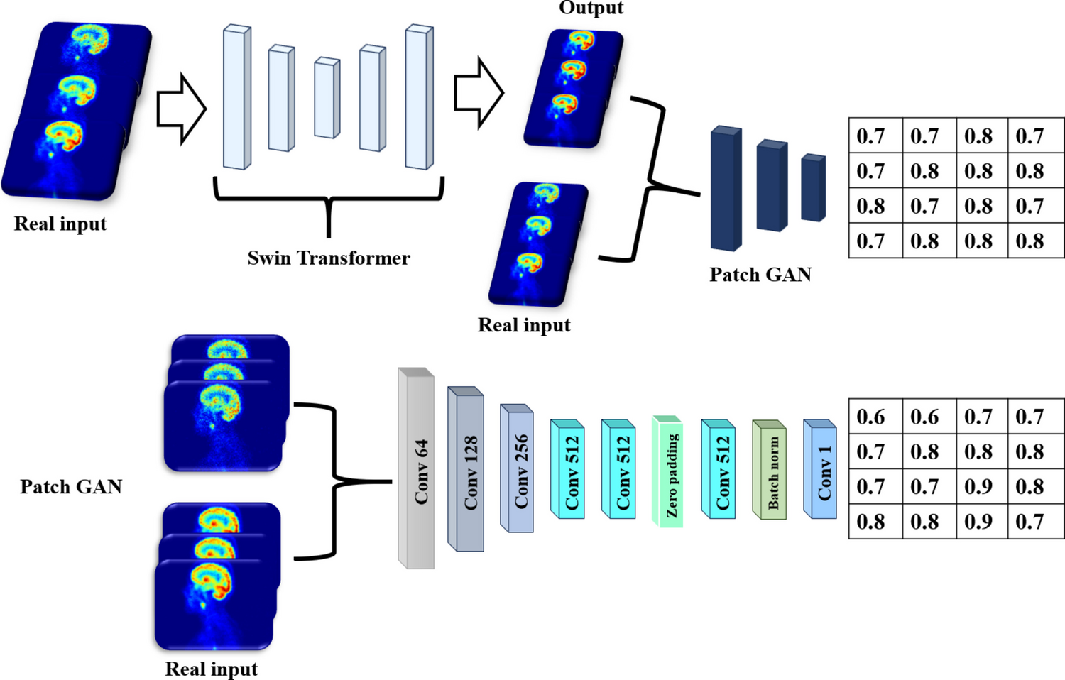
Network Architecture

The architecture of the proposed SwinPix network is illustrated in Fig. 1. Built upon the Pix2Pix framework, SwinPix replaces the conventional convolutional generator with a Swin Transformer-based design, while preserving the PatchGAN discriminator to enforce patch-level realism. The generator follows an encoder–bottleneck–decoder structure with skip connections, which helps retain spatial details during down-sampling and improves anatomical fidelity in the reconstructed PET images.

Fig. 1

The proposed SwinPix architecture for PET image denoising using a generator and PatchGAN discriminator. The generator, based on a Swin Transformer structure, processes real low-dose PET images to output denoised, high-quality images. The PatchGAN discriminator evaluates smaller patches of the generated image, comparing them to real input patches to ensure realistic details in texture and structure. The generator retains skip connections between the encoder and decoder blocks to preserve spatial information that might otherwise be lost during down-sampling, while the discriminator uses a patch-based approach to enhance image sharpness and realism by assigning probability values to individual patches, as shown in the right grid

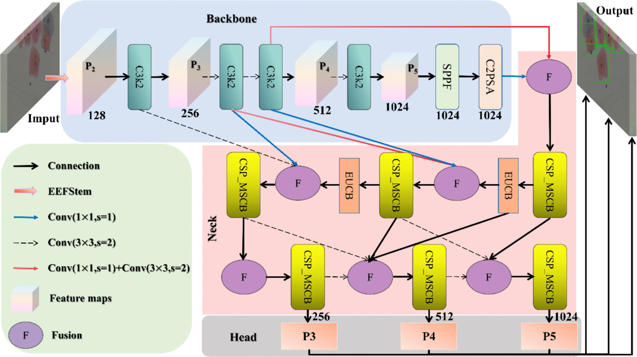
Specifically, the encoder consists of four hierarchical down-sampling blocks based on 3D convolutions and residual connections. The extracted feature maps are passed to a Swin Transformer bottleneck, which employs window-based self-attention and a shifted window strategy to capture both local texture information and global contextual dependencies. The decoder mirrors the encoder using up-sampling stages with skip connections to refine feature representations and restore image resolution. The discriminator adopts the standard PatchGAN architecture used in Pix2Pix, encouraging sharper and more realistic outputs. Since both the PatchGAN discriminator and the Swin Transformer shifted-window self-attention mechanism are well established, we refer readers to the original Pix2Pix and Swin Transformer publications for full architectural and mathematical details [49, 50]. For completeness, Fig. 2 provides an overview of the shifted-window attention mechanism employed in the Swin Transformer bottleneck.

Fig. 2

The graphical illustration of the Swin Transformer network. The architecture consists of an encoder-decoder structure, incorporating a bottleneck layer and transformer block for enhanced image feature extraction and reconstruction. The encoder blocks progressively down-sample the input image, while the decoder blocks perform up-sampling to restore the image resolution. A series of transformer layers, utilizing multi-head attention, facilitate global feature learning and contextual understanding. The architecture is specifically designed to improve image restoration tasks, such as PET image denoising, by leveraging both local and global dependencies in the image

To evaluate the impact of multi-input configurations, we trained both single-input and multi-input models at 4%, 6%, and 10% dose levels. Single-input models used only the target LD dataset (e.g., 6%), while multi-input models combined the target dose with auxiliary lower-dose inputs (e.g., 6% + 4% + 2% for the 6% case, 4% + 3% + 2% for the 4% case, and 10% + 8% + 6% for the 10% case). In all experiments, the ground-truth SD PET reconstructed from full-count data served as the reference for training and evaluation.

Loss Function

To enhance the performance of our network, we implemented a loss function that combines the Structural Similarity Index Measure (SSIM) and Root Mean Square Error (RMSE) and Adversarial Loss (GAN Loss). SSIM is a perceptual loss function that evaluates the similarity between input and output images by assessing luminance, contrast, and structural information. It is widely used in image processing to determine the quality of an image following compression, transmission, or other modifications. Unlike traditional methods, such as the Mean Squared Error (MSE) or Peak Signal-to-Noise Ratio (PSNR), which treat the image as a collection of independent pixels, SSIM takes into account changes in structural content, luminance, and contrast. The SSIM between two image windows \(X\) and \(Y\) is computed as follows:

$$SSIM\left(X,Y\right)=\frac__+_\right)\left(2_+_\right)}_^+_^+_\right)\left(_^+_^+_\right)}$$

(1)

μx and μy are the average of x and y.

\(_^\) and \(_^\) are the variances of x and y.

\(_\) is the covariance of x and y.

C1 and C2 are small constants to stabilize the division when the denominator is close to zero.

On the other hand, RMSE is a statistical measure commonly used to assess the difference between predicted values and actual observations. It is particularly useful in regression analysis, forecasting, and image processing to evaluate the accuracy of predictions or the quality of approximations. RMSE is calculated as:

$$RMSE= \sqrt\sum\nolimits_^_-\hat_\right)}^}$$

(2)

where:

n is the number of observations.

yi is the observed value.

\(\hat_\) is the predicted value.

In our approach, we define the SSIM loss as (\(_}=1-SSIM(X,Y)\)), and combine it with RMSE to form a comprehensive image loss function Limage. Here, \(I\) denotes the ground-truth SD PET image reconstructed from full-count data, \(\widehat\) represents the PET image predicted by the network, and \(_}\) refers to the voxel-wise summation term used for normalization in the RMSE and SSIM computations.

$$_ }\left(I,\hat\right)=RMSE\left(I,\hat\right)+0.6 \ast _} \left(I,\hat\right)$$

(3)

This function is used to optimize our network by minimizing the following loss:

$$\text=_ }\left(_},\hat\right)+ _ }\left(_},\hat\right)$$

(4)

This combined loss function balances structural fidelity and pixel-wise accuracy, leading to improved network performance in producing high-quality, denoised images. In the multi-input setting, the LD PET images at different dose levels (e.g., 4%, 3%, and 2%) were concatenated along the channel dimension and provided jointly to the network as input. The network then generated a single SD PET prediction, and the loss functions defined in Eqs. (3) and (4) were computed only on this output relative to the ground-truth SD PET image. Therefore, the formulation of the loss did not change between single- and multi-input settings; rather, the richer input representation allowed the model to exploit complementary noise realizations across dose levels.

The adversarial loss in the Pix2Pix model encourages the generator to produce images that are indistinguishable from real ones. This forces the generator to create outputs that can deceive the discriminator into classifying them as real.

Discriminator Loss: The discriminator’s goal is to differentiate between real and generated images. It does this by minimizing the binary cross-entropy loss, which ensures that the discriminator correctly classifies real images as real and generated images as fake.

The adversarial loss function is defined as:

$$_ \,\left(G,D\right)= _\left[\text\,D\left(x,y\right)\right]+ _[\text(1-D\left(x,G\left(x\right)\right))]$$

(5)

In this equation:

The discriminator (D) minimizes the first term, which corresponds to correctly identifying real images.

The generator (G) aims to minimize the second term, which encourages it to produce images that fool the discriminator into thinking they are real.

Thus, the adversarial loss for the generator is:

$$_\left(G\right)= _[\text(1-D(x,G\left(x\right)))]$$

(6)

Model training

The SwinPix was implemented using TensorFlow 2.8 on NVIDIA GeForce RTX 3060 (12 GB memory). The dataset, consisting of 219 PET/CT brain images, was divided into 150 images for training and 69 images for testing. Importantly, this division was performed strictly on a patient-wise basis, such that all dose-level reconstructions derived from the same subject were included exclusively in either the training or the test set. This ensured that no correlated dose renditions from a given patient appeared in both sets, preventing any data leakage during evaluation. For both training and evaluation, consistent dose-level configurations were used, and evaluation was performed only on unseen patients using the same input-dose setting as in training (e.g., a model trained with 10%, 8%, and 6% inputs was tested on held-out subjects using the same configuration). No cross-configuration testing (such as training with multi-inputs but testing with a single input) was performed to ensure consistency between training and evaluation settings. The network was trained over 20 epochs, with each epoch comprising 600 iterations. To prevent overfitting, we applied random rotations to the images before feeding them into the network. This simple augmentation strategy increases the diversity of the training set by exposing the network to different spatial orientations of the same anatomical structures. As a result, the model is less likely to memorize specific spatial patterns and instead learns more robust, rotation-invariant features. This variability effectively reduces overfitting and improves the generalization capability of the network when applied to unseen data. The training process utilized the Adam optimizer and a multi-loss function to assess the network's output against the ground truth labels. The learning rate was initially set at 0.001, with a batch size of 1. Throughout the training process, we ensured that the model did not overfit by monitoring the training loss and adjusting the learning parameters accordingly. The network's performance was validated on the test set to ensure generalization to unseen data.

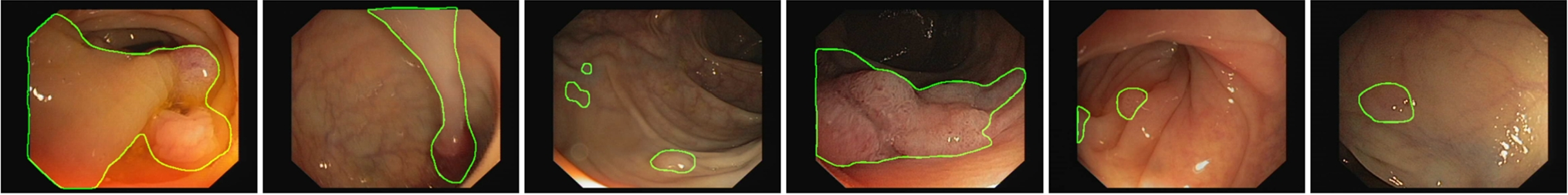
Evaluation Strategy

To assess the performance of various denoising models and the impact of incorporating prior knowledge from multiple LD PET images, we used five quantitative metrics. These included the SSIM, PSNR, and RMSE, calculated based on the standardized uptake value (SUV) for both the entire head region and malignant lesions. The test dataset included manually segmented lesions, outlined by nuclear medicine physicians during routine clinical procedures for diagnosis, lesion assessment, and treatment. Although lesion contouring was performed on PET images, CT structures were also considered during the identification process. Additionally, we computed the mean SUV bias (SUVmean bias) and maximum SUV bias (SUVmax bias) by comparing the predicted SD PET images to the reference SD PET images within the malignant lesions. Statistical analysis was performed in a repeated-measures framework because all reconstruction methods were evaluated on the same cohort of patients. For each quantitative metric, a one-way repeated-measures analysis of variance (RM-ANOVA) was conducted across models at each dose level. Upon significance, post hoc paired t-tests were carried out versus the LD baseline, with Holm correction applied to control the family-wise error rate over six comparisons per metric (p < 0.05).