In medical computed tomography (CT) imaging, metals appear in, for example, dental implants and orthodontic braces. Compared to biological tissues, metallic materials attenuate and scatter x-rays more strongly and highly non-uniformly across the x-ray energy spectrum, leading to inconsistent x-ray projections. These inconsistencies introduce severe streaking and shading artifacts in reconstructed CT images (De Man et al 1999, Boas and Fleischmann 2012, Gjesteby et al 2016), significantly degrading image quality and compromising downstream medical image analysis. Metal artifacts are often even more severe in cone-beam CT (CBCT) due to greater scatter, lower tube voltage, and cone-beam effects (Schulze et al 2011).

Metal artifact reduction (MAR) aims to mitigate these detrimental effects. From a reconstruction viewpoint, MAR algorithms can be grouped into three main categories: model-based iterative reconstruction (MBIR-MAR), image-domain MAR (ID-MAR), and projection-domain MAR (PD-MAR). Notably, most MAR methods in the literature address the 2D CT setting rather than 3D CBCT (Schulze et al 2011, Boas and Fleischmann 2012).

MBIR-MAR methods combine a physics-based observation model with image priors in an iteratively solved optimization problem. They can produce excellent results and provide a principled way to incorporate prior information, e.g. sparsity-driven approaches (Choi et al 2011), total variation with inequality constraints (Schiffer 2018), and polychromatic statistical reconstruction (Bismark et al 2020). However, MBIR approaches are typically computationally expensive due to repeated reconstruction and forward projection, limiting its practical impact.

ID-MAR methods apply post-processing to reduce streaks in reconstructed images (Zhang and Yu 2018, Liang et al 2019, Liao et al 2019, Khaleghi et al 2021). Because they operate after reconstruction, lost or distorted structures may be difficult to recover with high fidelity.

PD-MAR methods act on the projection data before reconstruction by identifying metal-corrupted regions and completing the corresponding projections. Many PD-MAR approaches treat the corrupted measurements as missing data and perform data completion using neighboring information. Although interpolation-based methods are computationally efficient, interpolation errors in the sinogram can lead to secondary artifacts in the corrected reconstructions (Meyer et al 2010, Boas and Fleischmann 2012). Normalized MAR methods mitigate this issue by interpolating normalized projections using a prior image (Meyer et al 2010, 2012). After projection completion, a metal-only reconstruction can be inserted into the artifact-reduced one to obtain the final result.

PD-MAR is often viewed as consisting of two steps: (1) metal segmentation and (2) inpainting. Accurate segmentation is critical, and simple thresholding is often insufficient (Boas and Fleischmann 2012). After segmentation, inpainting can be performed using either traditional algorithms or learning-based approaches.

Metal segmentation can be performed in either the image or sinogram domain. ID segmentation is more intuitive and commonly used in practice. The most straightforward approach is thresholding to isolate high-attenuation regions, for example using adaptive thresholding (Bernsen 1986, Niblack 1986, Sauvola and Pietikäinen 2000). While fast and simple, thresholding is sensitive to beam hardening and artifacts and may fail with overlapping tissues or metals of varying densities. In CBCT, where Hounsfield unit (HU) values are less reliable than in CT, thresholding can also yield inaccurate metal boundaries. Nevertheless, a common workflow is to threshold in the image domain and forward project the resulting metal mask to obtain a metal trace in the sinogram. For example, (Lee et al 2020) uses ID thresholding in dental CT before applying a fully connected network to refine a linearly interpolated sinogram. Atlas-based segmentation (Rohlfing et al 2004) can leverage anatomical priors, but requires accurate registration and may be brittle in complex cases.

Most PD-MAR methods therefore segment metal in the image domain and forward project the mask to the sinogram. Direct segmentation in the projection domain is comparatively less explored and also challenging: simple thresholding can be ambiguous due to overlaps and path-dependent attenuation, producing non-uniform and view-dependent metal traces. Nevertheless, addressing metal segmentation (and inpainting) directly in the projection domain is appealing, since it avoids introducing artifacts during reconstruction and allows the sinogram geometry to be exploited analytically.

Deep learning-based PD-MAR methods have become popular, see, e.g. Ghani and Karl (2019), Gomi et al (2019), Lee et al (2020), Agrawal et al (2021). In many settings, learning-based MAR improves quantitative performance relative to classical approaches, although methods operating solely via sinogram enhancement tend to underperform ID approaches (Gjesteby et al 2016). As an example, (Ghani and Karl 2019) proposes a conditional GAN for security CT, where metal is segmented by ID thresholding followed by morphological operations, then forward projected to generate a sinogram mask; the contaminated projections are removed from the original sinogram.

Machine learning-based segmentation methods, such as CNNs or U-Nets trained on real (Hegazy et al 2019) or synthetic (Agrawal et al 2023) CBCT data, can generalize across noise levels and artifact patterns. However, they require annotated training data and careful model development, and may be less transparent than analytical approaches. Moreover, in clinical environments, reliance on machine learning can increase regulatory complexity and approval timelines, since AI solutions are often classified as high-risk medical devices and are subject to evolving regulatory requirements across jurisdictions (e.g. MDR and the EU AI Act in Europe) (Aboy et al 2024). Consequently, where feasible, conventional non-learned algorithms may be advantageous.

Despite the appeal of PD MAR, most PD-MAR methods still rely on ID segmentation followed by forward projection to identify corrupted sinogram regions. This motivates analytical methods that perform robust segmentation directly in the projection domain.

To segment metals directly from the 3D sinogram, we propose a method based on the three-dimensional dual-tree complex wavelet transform (3D DT-CWT), which extends the DT-CWT to three dimensions (Wang et al 2007, Chen and Kingsbury 2012). The 3D DT-CWT provides approximate shift invariance and directional selectivity, which are useful for analyzing 3D sinogram volumes. While the 2D DT-CWT has previously been used within iterative CT reconstruction for MAR (Us et al 2019), here we use the 3D DT-CWT to computationally extract the wavefront set corresponding to metal objects in the CBCT 3D sinogram volume, followed by morphological processing to obtain a segmentation. After segmentation, inpainting is performed in the projection domain to complete the MAR pipeline. We evaluate the method on clinical scanner data, including both clinical acquisitions and simulated metals.

The main novelty of this work is the use of the 3D DT-CWT for direct analytical metal segmentation, enabling extraction of metal traces from volumetric projection data without ID thresholding or learned models. 3D DT-CWT provides approximate shift invariance together with strong directional selectivity in three dimensions, enabling robust extraction of metal features directly from the 3D sinogram. This is particularly beneficial in CBCT, where metal traces propagate continuously across projection angles and slices. Unlike CNN-based segmentation methods, the proposed framework is fully analytical and training-free, requiring no annotated datasets or retraining across scanners or acquisition protocols. In contrast to previous 2D DT-CWT-based MAR approaches, where the transform was incorporated within iterative reconstruction algorithms, our method applies the 3D DT-CWT directly to the full 3D CBCT sinogram volume for PD metal segmentation. This enables exploitation of the volumetric geometric continuity of metal traces across projection views, which cannot be captured by independent 2D processing.

The remainder of the paper is organized as follows. Section 2.1 reviews the framework of CBCT. Section 2.2 introduces the DT-CWT and describes its use for singularity extraction. Section 2.3 presents the proposed MAR method step-by-step. Section 2.4 describes the comparison method based on ID hard thresholding (HT). Section 2.5 describes the simulated and experimental datasets. Section 2.6 details the quantitative evaluation metrics, and section 3 presents the results. Finally, sections 4 and 5 conclude with a discussion and directions for future work.

2.1. CBCT

CBCT is a lightweight and low-cost alternative to conventional CT. In CBCT, the patient is scanned using a cone-shaped beam and an x-ray detector panel for direct 3D image reconstruction. The 2D projection images of the field of view (FOV) are acquired during a single rotation. CBCT scanning cuts the radiation exposure when compared to helical CT, as the scanning FOV is smaller and tightly cropped (Kalender 2011). Common applications of CBCT are dental imaging (Kiljunen et al 2015), extremity imaging and orthopedic studies (Pla n.d.), and oral and maxillofacial imaging (Angelopoulos et al 2012).

The benefits of CBCT are its mechanical simplicity, mobility, low cost, and high spatial resolution compared to conventional CT. However, the cone-shaped x-ray beam, slow rotation, and limited detector area may lead to artifacts and low temporal resolution. Furthermore, the increased scattering with CBCT produces inferior soft-tissue contrast, magnified metal artifacts, and poor HU stability, which have limited the widespread applicability of CBCT (Kiljunen et al 2015). Metals are a significant source of artifacts in dental CBCT, which complicates clinical decision making (Bamberg et al 2011). To address these challenges, novel reconstruction algorithms and MAR algorithms tailored for CBCT are needed to increase diagnostic image quality (Mahnken et al 2003, Wei et al 2004, Bal and Spies 2006, Prell et al 2009).

The projection data in CBCT imaging forms a 3D -volume, also referred to as the 3D sinogram. Each -plane corresponds to a single 2D projection image, and the projection angle proceeds along the -axis. Each -plane of the 3D projection data superficially resembles a conventional 2D sinogram. However, only data from the midplane, perpendicular to the axis of rotation and containing the x-ray point source, is a true sinogram in the sense of containing the Radon transform of the object in that plane (Schulze et al 2010).

CBCT geometry requires demanding reconstruction mathematics. The key problem with exact 3D reconstruction is that the 3D sinogram does not represent a Radon space. There is a method to overcome this problem, but still, the assumption is that a complete set of Radon data is available (Buzug 2009). For the popular circular x-ray trajectory used in most technical applications, a complete set of Radon data is not available. Luckily, there are approximation methods that can also deal with incomplete Radon data. The most frequently used method for cone-beam reconstruction is the Feldkamp–Davis–Kress (FDK) algorithm (Feldkamp et al 1984), which is an approximate extension of the 2D filtered backprojection algorithm into 3D cone-beam geometry.

2.1.1. Metal artifacts in CBCT

Metals in the scanned object cause inconsistencies in the projection data, resulting in artifacts in the reconstruction. Metal artifacts typically appear as bright or dark streaks surrounding metal objects in the CBCT image, as dark regions between metal objects, and as cupping effects. The inconsistencies are due to a number of mechanisms, most importantly beam-hardening, scatter, noise, photon starvation, the non-linear partial volume (NLPV) effect, and aliasing (De Man et al 1999, Boas and Fleischmann 2012, Gjesteby et al 2016). The ramp filtering and backprojection in FDK reconstruction spread these inconsistencies into global artifacts. Compared to CT, metal artifacts are exacerbated in CBCT (Schulze et al 2011).

The standard reconstruction model in x-ray tomography is based on Beer–Lambert law, where the x-ray intensity registered at detector pixel is

where is the intensity of incident x-ray beam and is the distribution of attenuation coefficients in the object. However, clinical scanners use polychromatic x-ray sources, and the attenuation model must be extended to

Metals attenuate different x-ray energies highly nonlinearly, and lower energy photons experience extremely strong attenuation, and the average beam energy increases, i.e. hardens, as it passes through the medium. Furthermore, due to beam-hardening, the ratio of photoelectric absorption and Compton scattering changes for the remaining higher energy photons, with Compton effects dominating. As a result, photon paths are altered and they are registered at the detector off the center line of the incident beam. These effects causes strong inconsistencies in the observed integral attenuation values. If photon starvation occurs, practically all photons along a given ray path are absorbed and very strong streak artifacts arise.

Metals can cause a very high portion of the incident radiation to be absorbed. Due to low photon counts, the signal registered behind metals is very noisy as result of photon Poisson statistics and detector electronic noise. The random noise effects are propagated across the image during reconstruction, resulting in streaking artifacts.

The finite detector pixel size and reconstruction grid size can lead to NLPV effects when a metal object only partially covers a given voxel, resulting in incorrect attenuation estimation. The finite number of projection directions can also lead to streak-like artifacts around metals due to aliasing.

2.2. 3D DT CWT

Analogous to Fourier analysis, wavelet methods decompose a function into translated and scaled copies of a mother wavelet. Wavelets have proven highly effective in signal processing applications, such as image compression. However, standard discrete wavelet transforms (e.g. Haar or Daubechies) suffer from shift sensitivity and exhibit poor directional selectivity, particularly in higher dimensions. The DT CWT (Kingsbury 1998, Selesnick et al 2005) addresses these limitations by employing two parallel wavelet decompositions, which can be interpreted as the real and imaginary components of a complex-valued transform. This DT construction yields approximate shift invariance and significantly improved directional selectivity, providing 28 distinct directions in three dimensions.

The 3D DT-CWT consists of complex-valued scaling and wavelet functions. Consider a complex, approximately analytic wavelet , defined by

where and are the real and imaginary parts of , respectively, and associated with a high-pass filter . Similarly, a complex scaling function is given by

and associated with a low-pass filter . The real parts and correspond to the real components of the wavelet and scaling function, while and are the imaginary components. For computational purposes, we use finitely supported wavelets, yielding approximately analytic wavelets.

We define the complex wavelet coefficients by

where represents the scale and denotes the spatial index. The index represents the oriented subbands, and there are 28 distinct directional subbands at each scale , indexed by:

These 28 subbands represent the high-pass (detail) information in the transform, oriented in different directions along the three spatial dimensions. The subbands correspond to combinations of separable high-pass filters across the three axes, with each of the 7 fundamental orientations being replicated across 4 distinct quadrants (combinations of positive/negative real and imaginary parts).

The 3D wavelets are constructed as tensor products of the 1D scaling and wavelet functions. For example, the wavelet in the subband is defined by:

Similarly, for a conjugate subband, such as , we have:

In this manner, each of the 28 subbands corresponds to a distinct combination of wavelet functions along the three coordinate axes, yielding directional wavelets with high selectivity in 3D.

For discrete 3D images of size , the indices range from to for each scale . The transform starts at the finest scale, applying the analysis filters to the voxel data, and proceeds toward coarser scales by filtering the low-pass subbands.

The function can be reconstructed from its coefficients via:

where is the frame operator, with being the analysis operator and the synthesis operator.

2.2.1. Wavelets in singularity extraction

The wavefront set characterizes both the spatial locations and the orientations of singularities of a function. Let . We say that is microlocally smooth at if one can find a cutoff function with such that the Fourier transform of the localized function decreases faster than any polynomial in as . If no such rapid decay occurs, then lies in the singular support of .

Directional information is obtained by examining the decay of the localized Fourier transform within angular regions of the frequency domain. If decay is not rapid inside a conical neighborhood centered at direction , then is an element of the wavefront set . In imaging problems, corresponds to the local edge orientation perpendicular to an interface.

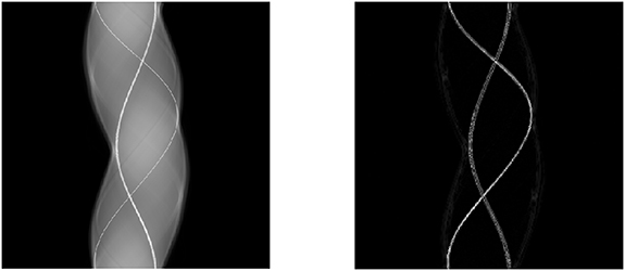
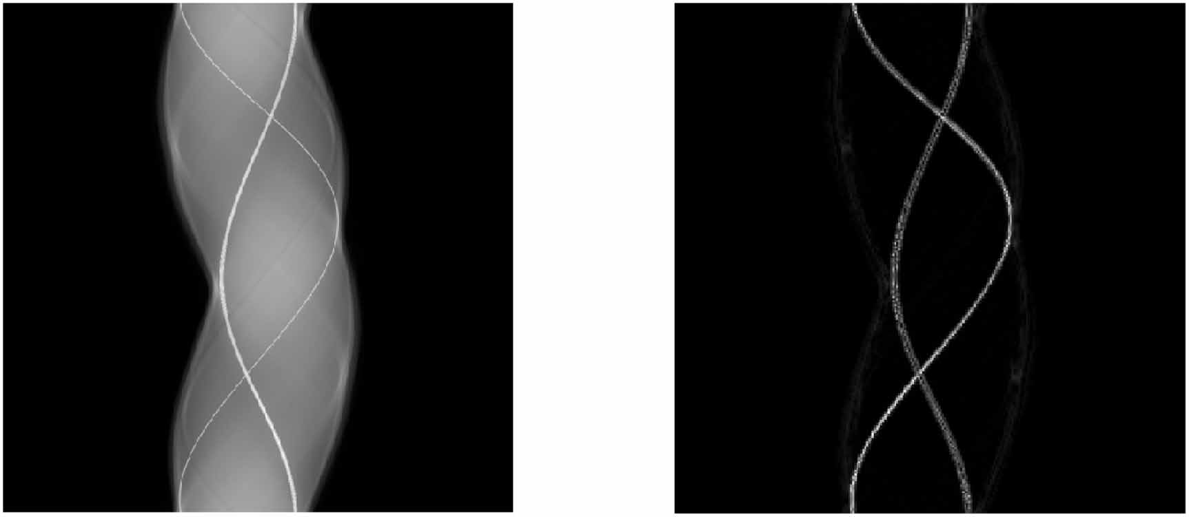
In practice, the CWT is an effective tool for extracting singularities from a signal, as previously demonstrated for CT wavefront set extraction in Rautio et al (2023). In images and volumetric data, large-magnitude wavelet coefficients typically occur near jumps and edges. See figure 1 for an example of a sinogram containing two metal inserts, where the sum of the absolute values of the wavelet coefficients reveals the corresponding metal boundaries.

Figure 1. Sinogram (left) and the sum of the absolute value of the largest complex wavelet coefficients, revealing the location of the metals (right).

Download figure:

Standard image High-resolution image

The DT-CWT offers directional selectivity with moderate redundancy and computational efficiency. Real-valued wavelets provide only limited orientation discrimination, while curvelets (Candès and Donoho 2004) and shearlets (Labate et al 2005, Kutyniok and Labate 2012) achieve finer directional resolution at increased computational cost. For large 3D volumes, the DT-CWT provides a suitable balance between directionality and computational feasibility.

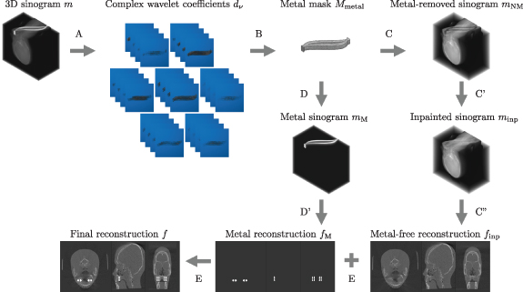
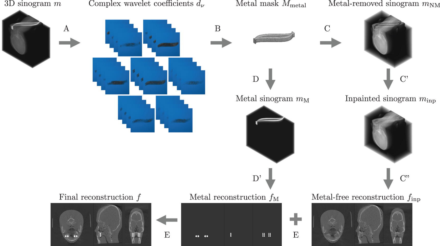
2.3. Proposed PD MAR method

We propose a MAR method for PD metal segmentation and inpainting, that uses 3D DT-CWT to find the edges of metals in the 3D sinogram. Figure 2 shows the full workflow from 3D sinogram to metal artifact reduced reconstruction. The method is explained in detail below.

Figure 2. The proposed workflow for metal artifact reduction, based on projection-domain metal segmentation. Steps include: (A) Extracting the wavefront set related to metals from the 3D sinogram. (B) Binary mask for metal segmentation. (C) Sinogram inpainting and metal-free reconstruction. (D) Metal reconstruction. (E) Final result: combining the artifact-free inpainted reconstruction and metal reconstruction.

Download figure:

Standard image High-resolution image 2.3.1. Extracting the wavefront set related to metals

We start with the 3D sinogram as the input, and take the DT-CW transform of it, resulting in 28 detail coefficient subbands , where is the subband index and is the number of voxels. In this work, only the first decomposition scale, , is used. The DT-CWT was computed using MATLAB’s ‘dualtree3’ implementation with the default first-level biorthogonal filters and a 10-tap Hilbert Q-shift filter pair.

Metals are highly attenuating, so they correspond to large wavelet coefficient values. We threshold away the smallest coefficients related to noise and non-metal features, by keeping only the largest coefficient values:

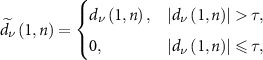
where is an empirically selected threshold applied to the normalized wavelet coefficients.

Note that coefficient thresholding might not fully eliminate non-metal contributions, since superimposed structures in the 3D sinogram may also generate singularities detected by the DT-CWT, potentially leaving residual coefficients in the subbands . This will be addressed in the next step.

2.3.2. Binary mask for metal segmentation

To move from the complex wavelet coefficient space to the 3D sinogram space , we take a sum over the absolute value of the thresholded coefficients:

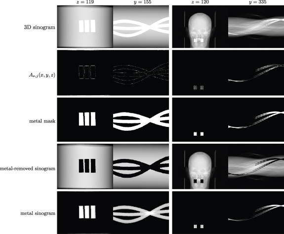
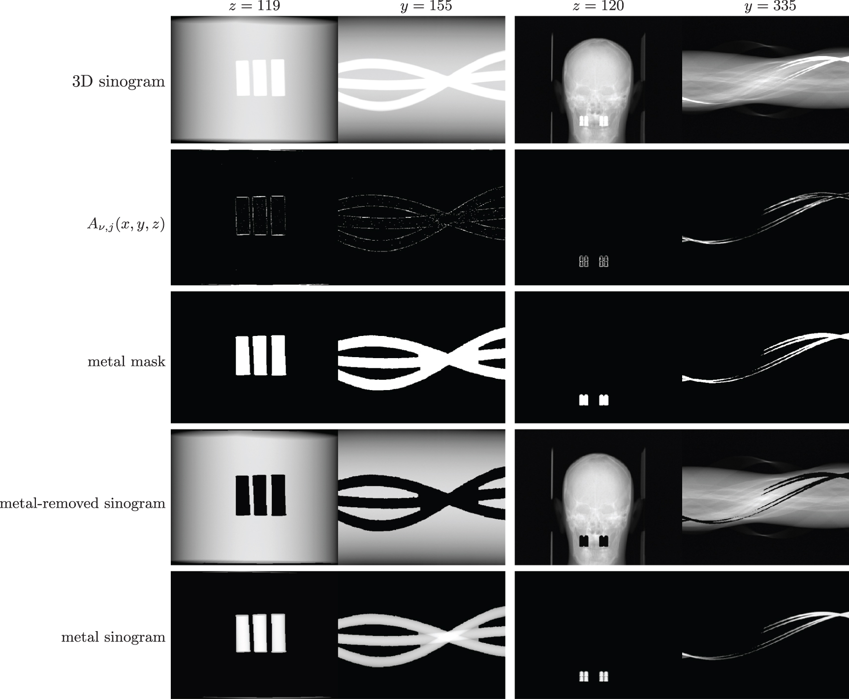
revealing the locations in the 3D sinogram space corresponding to the largest coefficients. See the 2nd row of figure 3 for an illustration of the resulting point cloud for two different 3D sinograms. Then, the result is binarized to by:

where denotes the indicator function.

Figure 3. Metal segmentation results for simulated cases (I) and (II), presenting - and -slices of the 3D CBCT sinograms. Note that the metal mask slightly overshoots the metal area over the neighboring slice due to the morphological closing operation.

Download figure:

Standard image High-resolution image

As mentioned in the previous subsection, the binary point cloud might still have voxels that are not related to a true metal trace, due to superimposition of features in the 3D sinogram. To remove these residuals, we leverage the geometric structure of sinograms and discard isolated voxels that do not align along a continuous geometric trajectory in the -direction. That is, a voxel is retained only if it has nonzero support within an