Since the introduction of the Bessel beam in 1987 [1], the potential utility of so-called ‘diffraction-free’ monochromatic beams [2, 3] in long-distance propagation has been of continued interest, with potential applications in free-space communications. The experimental tests carried out to date have demonstrated propagation distances typically on the order of meters [4–7]. Exceptions include 1 km experiments making use of a Bessel-like beam with controlled wavefront spherical aberrations [8], and most recently using an auto-focusing beam (a circularly symmetric Airy beam at a wavelength of 532 nm) whose initial 6-mm-diameter peak extends to 9 mm after 1 km [9].

We have recently investigated a family of propagation-invariant (diffraction-free and dispersion-free) pulsed beams dubbed ‘space-time wave packets’ (STWPs) [10–21], which are an outgrowth from extensive previous study of so-called ‘localized waves’ [3, 22–24]. STWPs are endowed with angular dispersion (AD) [3, 25]; i.e. each wavelength travels at a prescribed angle with respect to the propagation axis. In contrast, conventional tilted pulse fronts [26] are also endowed with AD, but are not propagation invariant. We have recently uncovered that the AD undergirding STWPs is ‘non-differentiable’; i.e. the derivative of the propagation angle with respect to wavelength is not defined at a particular wavelength [27–29]. The non-differentiability of the underlying AD profile is the key to the unique attributes of STWPs, rendering them distinct from tilted pulse fronts [29, 30]. Besides propagation invariance, STWPs have tunable on-axis group velocity [14, 15, 31, 32], group-velocity dispersion [33], and axial acceleration [34–39], and they exhibit self-healing [40] and anomalous refraction phenomena [41]. Furthermore, STWPs are readily synthesized in the paraxial regime without needing ultrabroad bandwidth sources as needed in propagation-invariant X-waves [22] or focus-wave modes [23, 42, 43].

Initial demonstrations of STWPs verified propagation invariance over small distances, which are nevertheless significantly larger than the Rayleigh range of a Gaussian beam having the same initial spatial width [12, 44]. We have increased the propagation distance of STWPs from mm in [12], to m in a laboratory environment [45], and m after directing the beam out of the laboratory and down a service chase in our research building [46]. Our previous work theoretically predicted the possibility of extending to the kilometer range.

Here we report on propagation measurements for STWPs over km in the open environment of a laser range in Florida (TISTEF: Townes Institute Science and Technology Experimentation Facility). We first establish a theoretical model that accounts for the various factors that limit the propagation distance of an STWP. Based on this model we synthesize STWPs at a wavelength nm and bandwidth nm. The transverse width of one STWP expands from mm to mm after 500 m; a Gaussian wave packet expands over the same distance to mm (Rayleigh range m). The width of another STWP expands from mm to mm after 1 km; a corresponding Gaussian wave packet expands to mm ( m). Our model points to the improvements required to extend .

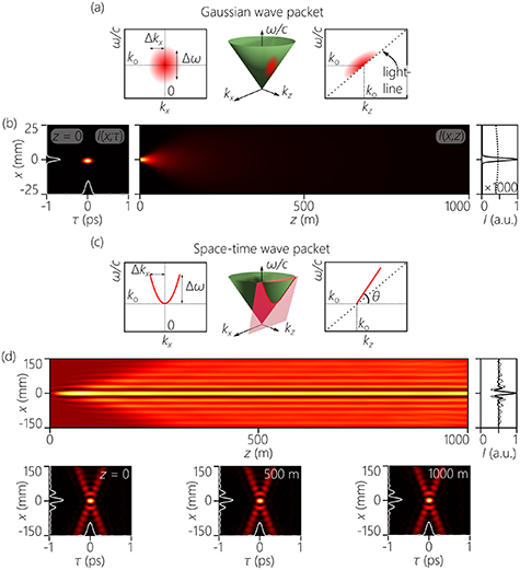
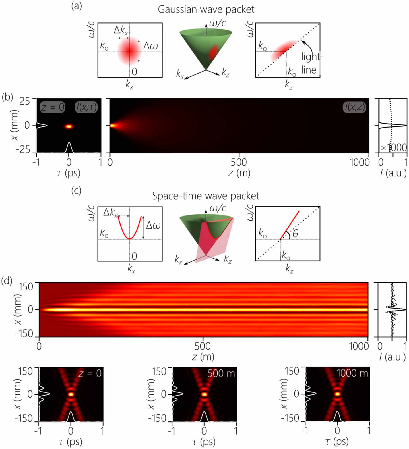
We compare conventional Gaussian wave packets (pulsed beams) in which the spatial and temporal degrees of freedom are separable, and STWPs in which they are not. We write the field in terms of a carrier and slowly varying envelope, , where is a carrier frequency, , and is the speed of light in vacuum. Here, we use only one transverse spatial dimension, , and hold the field uniform along . Recent developments have enabled the synthesis of STWPs modulated in both and [17, 47, 48], and we will use them for long-distance experiments in the near future. The envelope of the Gaussian wave packet is:

where and are the transverse and axial wave numbers, respectively, , and the spatio-temporal spectrum is the 2D Fourier transform of . The spectral support of such a wave packet is a 2D domain on the surface of the light-cone associated with the free-space dispersion relationship , and the spectral projections onto the and are also 2D domains (figure 1(a)). The spatio-temporal spectrum of conventional wave packets is typically separable , which is manifest in the initial spatio-temporal intensity profile (figure 1(b)). In the narrowband, paraxial regime we have 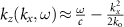, which leads to dephasing of the spatial frequencies along , and thus diffraction of the time-averaged intensity (figure 1(b)).

Figure 1. (a) Representation of the spectral support for a separable pulsed Gaussian beam on the surface of the light-cone, along with spectral projections onto the and planes. (b) Spatio-temporal profile of the pulsed Gaussian beam at , and the time-averaged intensity . Here rad/mm, mm, nm, nm, fs. The rightmost panel depicts at (solid) and at m (dashed). (c), (d) Same as (a), (b) for an STWP with , nm, and all other parameters are the same as for the pulsed Gaussian beam; in (d), is shown at , 500 m, and 1 km.

Download figure:

In contrast, the spatio-temporal spectrum of STWPs is not separable, and ideally a one-to-one relationship between and is enforced such that 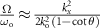, and thus , which is equivalent to restricting the spectral support on the light-cone to a 1D trajectory at its intersection with a plane making an angle (the spectral tilt angle) with the -axis (figure 1(c)). The STWP envelope takes the form:

which travels rigidly in free space at a group velocity [32]. The spatio-temporal intensity profile is X-shaped in any axial plane in this ideal limit (figure 1(d)).

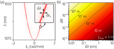
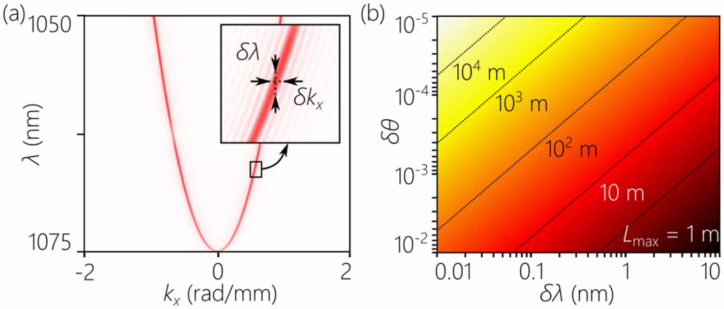
However, the ideal delta-function correlation between and (figure 1(c)) cannot be attained in practice because it implies an infinite energy. Instead, a finite spectral uncertainty arises in the association between and (figure 2(a)), in which case , where is a narrow function of width , and is the spatial frequency associated with in the ideal limit (in absence of spectral uncertainty). The spatial uncertainty is associated with a spectral uncertainty via (figure 2(a)). Thus, rather than a mathematical parabola, the spatio-temporal spectrum projected onto the -plane has a finite ‘thickness’: each spatial frequency is associated with a finite temporal bandwidth . This spectral uncertainty is one of the two key parameters that determines the propagation distance for an STWP, the other being : [44]. To increase one must reduce and have ; corresponds to a plane-wave pulse [49]. Defining an offset in the spectral tilt angle , we have for small and [46]; see figure 2(b).

Figure 2. (a) Calculated spatio-temporal spectrum of an STWP with mm and , highlighting the spectral uncertainty and spatial uncertainty in the inset. (b) Calculated propagation distance with the spectral uncertainty and offset in spectral tilt angle .

Download figure:

To set the stage for the measurements, we first compare the optical resources used to construct an STWP with those used to construct a pulsed Gaussian beam, against which it will be referenced. By optical resources, we mean the spatial bandwidth and the temporal bandwidth (or ) used. In the course of our experiments, we ensure that both the spatial and the temporal bandwidths of the pulsed Gaussian beam are equal to those for the STWP. The only difference between these two pulsed beams (or wave packets) is the following: whereas the spatial and temporal degrees of freedom are separable in the case of the pulsed Gaussian beam (its spatiotemporal spectrum separates into a product of a purely spatial spectrum and a purely temporal spectrum), the STWP—on the other hand—is not separable with respect to them (the spatial and temporal frequencies are tightly correlated; equation (2)). This is made clear by comparing the spatiotemporal spectrum for the Gaussian wave packet in figure 1(a) to that for the STWP in figure 1(c).

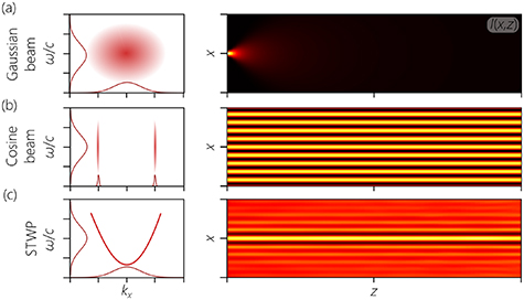
We plot in figures 3 and 4(a) comparison of different pulsed fields that illustrates the consequences of introducing tight spatiotemporal spectral correlations into the field for its axial propagation dynamics. Figure 3 compares three distinct optical fields in which the transverse spatial profile is localized along one dimension and is uniform along the other (i.e. in the form of a light sheet), whereas figure 4 compares analogous field configurations in which the transverse spatial profile is localized in both transverse dimensions.

Figure 3. Comparison of the spatiotemporal spectrum and the axial evolution of the time-averaged intensity for (a) a pulsed 1D Gaussian beam; (b) a pulsed 1D cosine beam; and (c) an STWP in the form of a light sheet. Left column: Spatiotemporal spectrum projected onto the -plane. The 1D projections along the -axis and the -axis are the marginal spatial and temporal spectra, respectively. These marginal spectra are identical in (a) and (c). Right column: Time-averaged intensity . All three fields have the same temporal bandwidth and the same spatial bandwidth . Consequently, they have the same minimum transverse spatial feature size at .

Download figure:

Figure 4. Comparison of the spatiotemporal spectrum and the axial evolution of the time-averaged intensity for (a) a pulsed 2D Gaussian beam; (b) a pulsed Bessel beam; and (c) an STWP localized along all dimensions. Left column: Spatiotemporal spectrum . We also plot the spatial spectrum projected onto the -plane. Right column: Time-averaged intensity . In (a), we plot an iso-spectral-inte