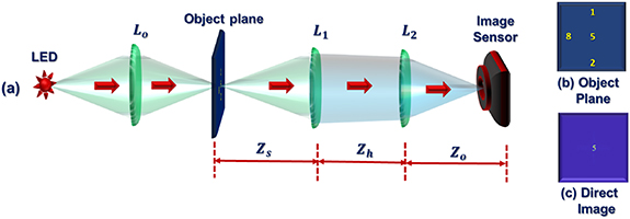
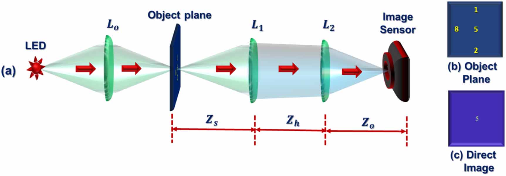
The descriptions of the optical system and the synthesis algorithm of the CPM in this section are valid for both the TMCA and the PSM, whereas the HSM is discussed in the next subsection. To illustrate the problem of a limited FOV, the optical configuration of a typical dual-lens imaging system without a CPM is shown in figure 1(a). The incoherent light emitted from the source illuminates the object through lens L0, and the transmitted light subsequently passes through lens L1 with focal length f1 positioned at a distance zs from the object plane. The resulting light is then relayed through lens L2, with a focal length of f2, placed at a distance zh from L1. The final intensity distribution is recorded by an image sensor located at a distance zo from L2. It is assumed that all the parameters, f1,2 and zs,h,o, satisfy the imaging equations between the camera and object planes. N = 4 separated objects positioned in the object plane are shown in figure 1(b), but although the illumination uniformly covers all the objects in figure 1(a), the presence of the lenses and the limited active area of the sensor result in capturing only the central object, as shown in figure 1(c), and the remaining objects fall outside the detectable region and thus remain unseen. The FOV of such an imaging system is equal to the ratio between the sensing size and the system magnification.

Figure 1. (a) Schematic of the optical imaging system. (b) Object plane, (c) resultant image in the camera.

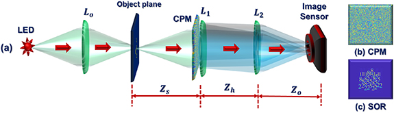
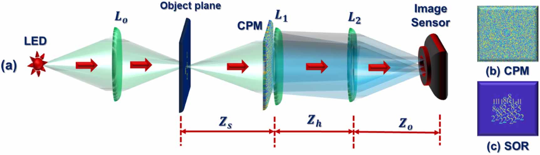
Download figure:

To bring all the objects’ images inside the sensing area, a CPM is attached to L1, as shown in figure 2. In the experimental setup, a phase-only spatial light modulator (SLM) is employed to display the CPM [26, 27]. For practical reasons, the product of the two-phase elements, the CPM and the lens, is displayed on the SLM as a single diffractive phase mask. In the case of the PSM, the CPM comprises a multiplex of N distinct scattering phase distributions, each corresponding to one of the N separated object areas. Each scattering phase is designed to generate a unique pattern of K sparse dots on the camera plane, which is considered the Fourier domain of the CPM [27]. In other words, the imaging system is configured so that the camera plane coincides with the Fourier plane of the CPM when the system is illuminated by a point source at the center of the object plane. This Fourier relation is due to the imaging conditions between the object and camera planes, and it allows the CPM to be synthesized using the Gerchberg–Saxton algorithm (GSA) [28].

Figure 2. (a) Optical imaging system for engineering the field of view. (b) CPM—coded phase mask, (c) System-to-Object response (SOR).

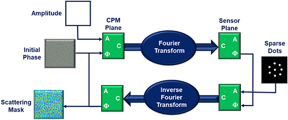
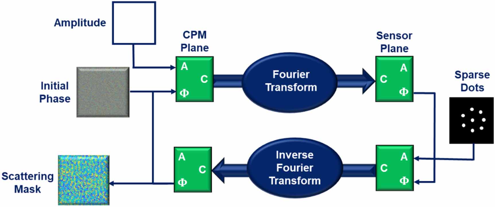
Download figure:

As mentioned above, each of the N scattering phase functions composing the CPM is synthesized via the modified GSA to independently operate on its corresponding object region, as illustrated in figure 3. The GSA is an iterative algorithm employed to generate distinct scattering phase distributions. In this algorithm, a uniform amplitude matrix and a random phase distribution within the range [0, 2π] are used as the initial inputs at the CPM plane. During each iteration, the amplitude of the Fourier transform of the CPM matrix is replaced by a predefined sparse dot pattern, while the corresponding phase information is preserved to compute the inverse Fourier transform. This process is repeated until the mean square error (MSE) between the original and obtained pattern of dots reaches stagnation, and the final phase distribution obtained at the CPM plane is extracted as the desired scattering phase function.

Figure 3. Schematic of the modified Gerchberg–Saxton algorithm.

Download figure:

The nth scattering phase is synthesized based on the spatial location of the nth object in the two-dimensional plane. Consequently, when only the nth scattering phase is displayed on the SLM (with the diffracted lens L1), K replicas of the nth object appear within the camera’s FOV. Simultaneously, the same scattering phase modulates light from the remaining N–1 objects, producing K replicas for each but positioned outside the sensor’s active region. Under the Fourier relationship between the CPM and the camera plane, these replicas are obtained outside the sensor because a corresponding linear phase is integrated into each nth scattering phase, in addition to the phase that is responsible for the central object region, which is inside the FOV of the system. During the GSA, the integration of a corresponding linear phase is achieved by shifting the constrained sparse dots of the nth scattering phase to the nth region on the sensor plane.

In the case of the TMCA, a single SLM is used to sequentially display different CPMs on all the SLM pixels. At time , CPM1 is displayed over the entire SLM, and the corresponding system-to-object response (SOR) is recorded. This process is repeated for N different CPMs to obtain N sets of PSFs and object response patterns, which are recorded one after another. Reconstruction is performed individually for each (PSFn, SORn) pair, and the resulting images are summed to obtain the final composite image.

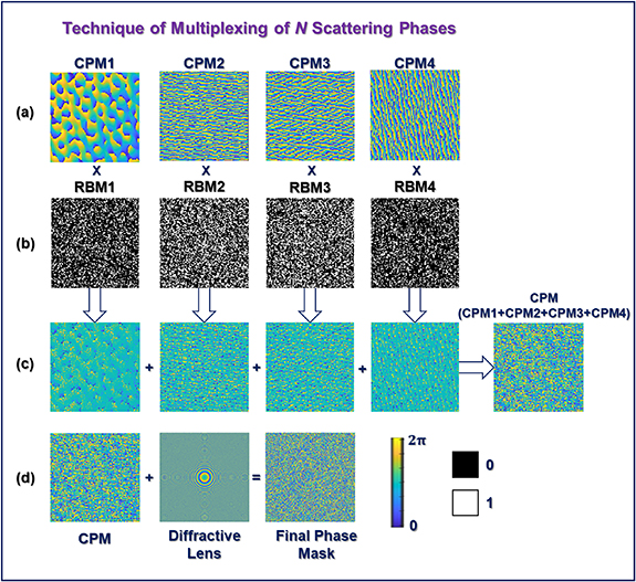
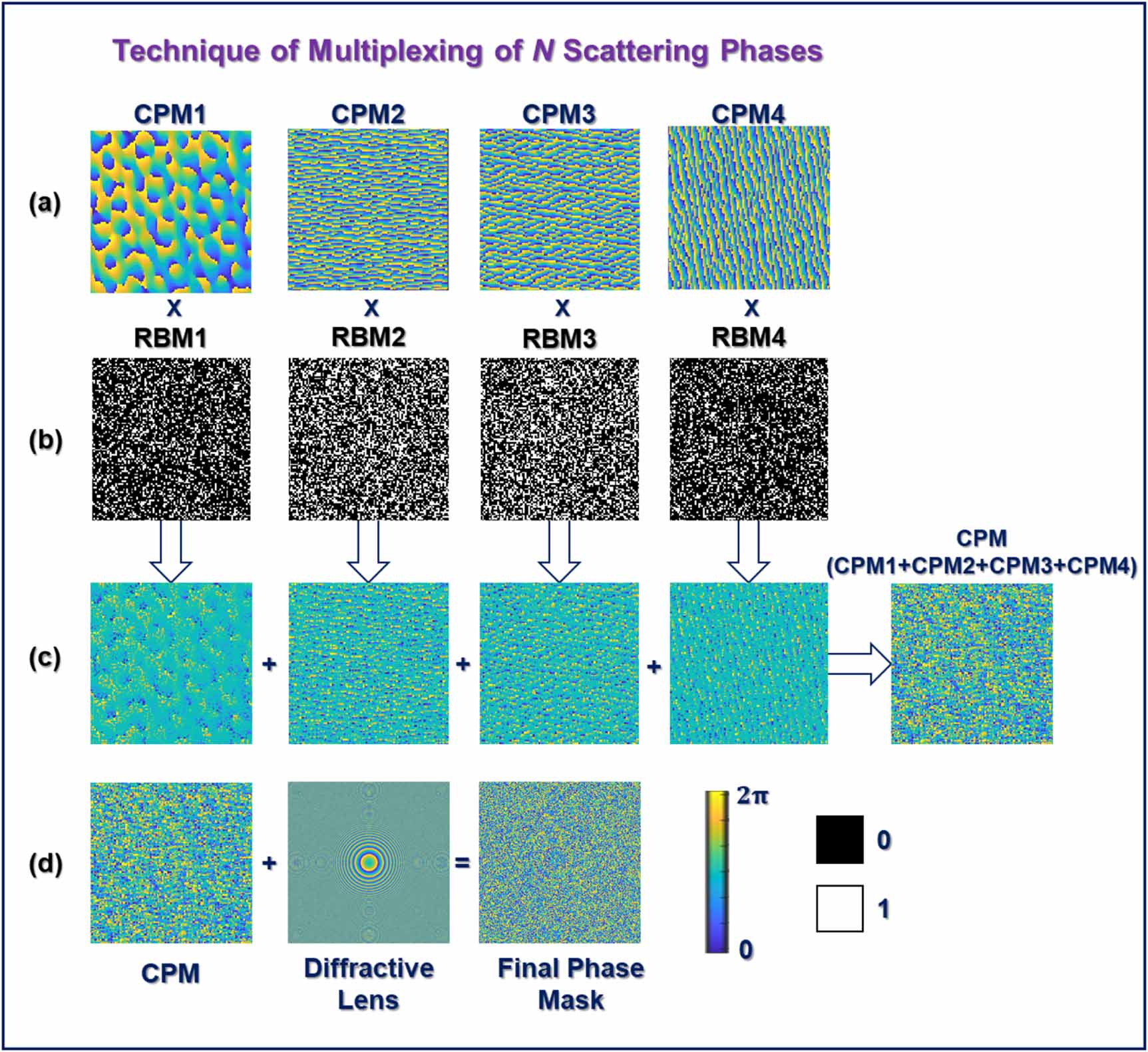
The main drawback of TMCA is obvious: one needs to record N SORs under N different CPMs, a slow process that may prevent the recording of a video of a dynamic scene. The single-shot PSM described here is one solution to the slowness of the TMCA, in which multiplexing is performed in space rather than in the time domain. The synthesis of N = 4 scattering phase distributions via the PSM is illustrated in figure 4. The four scattering phases synthesized via the GSA are shown in figure 4(a). N binary matrices in the range [0, 1] shown in figure 4(b) are created such that the locations of those are random, and the inner product of any two matrices is equal to the zero matrix. The inner products of the various scattering phases and random binary matrices are added to obtain the phase of the CPM in the PSM, as shown in figure 4(c). The resultant CPM is attached to the diffractive lens to satisfy the imaging condition between the object plane and the sensor plane. The final mask displayed on the SLM, which is the sum of the two phases of the CPM and the lens, is shown in figure 4(d). Consequently, the introduction of the CPM, formed by multiplexing all N scattering phases, into the optical system results in the formation of K distinct replicas of each of the N objects within the camera’s FOV. The representation of the CPM synthesized by the GSA is shown in figure 2(b) for the case of only N = 4 because in the PSM of N> 4, the reconstruction noise is too high to enable a reasonable quality of image reconstruction.

Figure 4. Multiplexing of N scattering phases by PSM: (a) four distinct scattering phases synthesized by the GSA; (b) four binary random patterns in which the inner product of any two different random patterns yields a zero matrix; (c) the product of four scattering phases with four random binary matrices is summed to obtain the phase of the CPM; (d) the phase of the CPM is added with the phase of a diffractive lens to obtain the final aperture phase mask. PSM—parallel spatial multiplexing, RBM—random binary matrix, CPM—coded phase mask.

Download figure:

In accordance with the scheme shown in figure 4, the synthesized CPM in the PSM is displayed on the single SLM, and the corresponding intensity response is recorded with a single camera shot. Image reconstruction is carried out on the single-shot SOR, which contains all the responses of N different scattering phases. The mathematical description of the FOV engineering is based on figure 2 and is valid mainly for the PSM. The goal of this analysis is to calculate the PSF of the system and formally verify that the FOV can be extended in postprocessing and in a flexible manner according to the user’s desire. The analysis is based on the Fourier relation between the CPM and the intensity distribution on the camera plane when the system is illuminated from a point at the center of the object plane. Since the system input is a point, the intensity in the output for the nth CPM (CPMn = is the nth PSF of the incoherent imaging system, given by

where and are the transverse location vectors in the camera and CPM planes, respectively. denotes the 2D Fourier transform operator, represents a scaling operator defined as , and zL is a parameter dependent on the location of the CPM in the system and the relevant parameters of the imaging system. is the limiting function of the aperture, usually given as , where R is the radius of the cone base of the beam incident on the CPM. In the present case, R is assumed to be the radius of the lens L1 in figure 5(a). The expression in equation (1) is a direct result of the imaging property of the system from the object to camera planes and, therefore, is valid for any incoherent imaging system regardless of the number of lenses and the position of the CPM in the system. The only factors that can be changed in equation (1), from one system to another, are the values of zL and the size of . Approximating the size of to infinity enables one to eliminate from equation (1) and from the entire analysis. Owing to the Fourier relation of equation (1), the PSFn obtained by the CPMn is synthesized by the GSA, as shown in figure 3, to yield K randomly distributed dots shifted to the nth region in the camera plane, formally given by

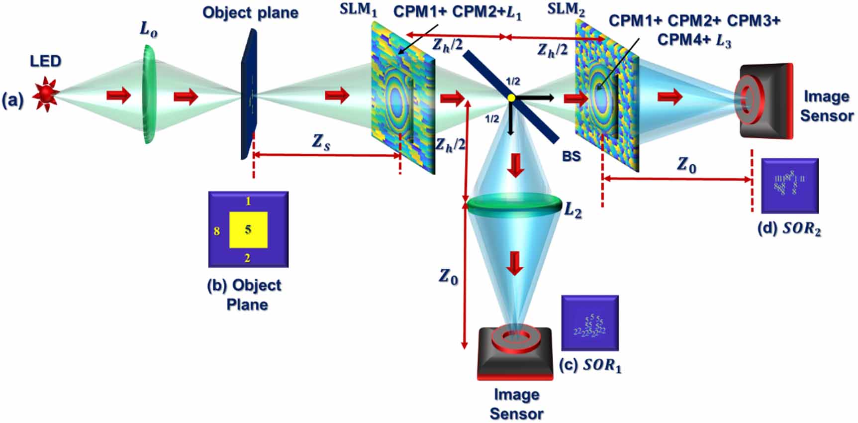
Figure 5. (a) HSM configuration for engineering the field of view. (b) Object (c) SOR1 and (d) SOR2.

Download figure:

where is the distance vector of the nth region center from the origin on the object plane, is the kth position of a dot in the set of K dots obtained by the GSA, is the convolution sign, δ is the Kronecker delta function, and M is the system’s transverse magnification. Owing to the shift of the dot pattern by the distance , when the input point is positioned in the center of the nth object region, a distance from the origin of the object plane, the dot pattern is guaranteed to be obtained at the center of the camera plane. In other words, the intensity response for a point object located at is

where zL =(zhf2-zhzo + zof2)/f2. zL can be easily calculated by choosing a mask , calculating the phase function at the camera plane, and extracting the constant of the linear phase exponent. According to equation (3), when the input point is positioned at the center of the nth object region, the corresponding PSF is formed at the center of the camera plane. The light originating from a point source in the nth object region, when modulated by the remaining (N–1) scattering phase masks, generates K(N–1) diffraction spots located outside the camera’s FOV. Consequently, the intensity distribution on the camera remains unchanged, as described in equation (3).

Next, the image reconstruction is analyzed. A two-dimensional object can be modeled as a sum of L shifted delta functions. Therefore, the intensity distribution on the object plane in the nth region of the object is

where is the transverse location vector in the object plane and represents the intensity at each spatial location. The corresponding intensity response recorded on the camera plane as a result of the object in the nth region is

equation (5) indicates that an object from the nth region on the object plane is duplicated K times and displayed around all the K dots of PSFn. For all objects, the total recorded SOR of the PSM is expressed as follows:

To reconstruct the object plane, both the recorded SOR and each are zero-padded. The zero-padded SOR is then deconvolved with the sum of the zero-padded and spatially shifted PSFs corresponding to each object region to avoid overlap of the individual object regions. The reconstructed image with an extended FOV is

where ⊛ denotes deconvolution in one of the commonly used techniques [29, 30] and where represents the spatial shift applied to the matrix to prevent overlap among the reconstructed objects. The reconstructed image , thus representing the superimposed contribution of all object images within the FOV, is retrieved by digitally deconvolving the recorded SOR with the ensemble of corresponding PSFs. Note that in the case of the TMCA, the nth object region is reconstructed via deconvolution between the nth SOR given in equation (5) and the nth PSF given in equation (3), such that the reconstructed image with an extended FOV is

Comparing equations (7) and (8), the cross-deconvolutions between SORn and PSFm (n ≠ m) in equation (7) are avoided in equation (8), leading to less noise in the images of the TMCA than those of the PSM.

The optical arrangement for the HSM configuration, which combines the principles of both parallel and serial spatial multiplexing to achieve a balanced trade-off between the acquisition speed, noise level, optical efficiency, and system complexity, is shown in figure 5. Owing to the cross-deconvolution between the nth PSF and the mth SOR (n≠ m) implied by equation (7), the image plane of the PSM has a relatively high level of noise between the reconstructed images. This spatial noise is reduced, although not completely eliminated, by reconstruction in TMCA, as implied by equation (8), because of the absence of the cross-deconvolutions mentioned above. However, TMCA is implemented by N camera shots for N object regions, making TMCA the slowest coded aperture multiplexing method. Compared with PSM and TMCA, the HSM is proposed as a single-shot multiplexing method, as fast as PSM, with reduced noise but at the cost of a greater degree of hardware complexity.

The HSM configuration shown in figure 5 uses only two SLMs and two image sensors arranged sequentially along the optical axis. In this setup, incoherent illumination from an LED uniformly covers the object plane containing spatially separated object regions. The transmitted light is first incident upon SLM1 and then SLM2. The system is designed to satisfy the imaging condition on the beamsplitter plane, a distance zh/2 from SLM1, SLM2, and L2. Hence, the conjugate phase of the CPM on SLM1 is projected onto SLM2. To enable proper modulation of the CPMs on SLM2 according to the design of the GSA, SLM2 should contain the CPMs of SLM1 in addition to the CPMs obtained by the GSA and the phase of L3. The total FOV of the HSM system is determined by the combined effective sensing areas of both channels and is identical to the results of the other multiplexing methods, PSM and TMCA.

To enable hybrid multiplexing, the total number of CPMs, in the present example, N = 4, is divided into two separate matrices, and each matrix is multiplexed by PSM (for 2 object regions) and displayed on a separate SLM. The phases of CPM1 and CPM2 are spatially combined to form the first composite mask (CPM1 + CPM2), which is displayed on the first SLM, whereas the phases of CPM3 and CPM4 are combined as (CPM3 + CPM4) and displayed on the second SLM. As mentioned above, because of the phase projection from SLM1, the total phase displayed on SLM2 is the sum of the phases of CPM1, CPM2, CPM3, CPM4, and L3. Each SLM with its subset of CPMs has a corresponding camera to record the resulting intensity response pattern, as shown in figure 5. The intensity responses from SLM1 and SLM2 are recorded simultaneously by two cameras placed at the same distances, one from L2 and the other from SLM2. Both cameras are in the image plane in relation to the beam splitter plane, which is also located in the image plane in relation to the object plane. Consequently, the transverse magnifications of both channels are zo/zs. Each camera, therefore, captures a superposition of SORs corresponding to the CPMs displayed on its associated SLM. As a result, the HSM approach achieves the simultaneous acquisition of multiple SORs within a single exposure with more optical components than in the PSM and TMCA but less image noise than in the PSM and faster acquisition than in the TMCA.

The intensity response of the dual-channel imaging system for a point object located at is

where c = 1 and c = 2 denote the two imaging channels of the proposed HSM. The SOR recorded simultaneously by the two imaging channels is expressed as follows:

Each imaging channel is independently reconstructed using its corresponding PSF, as represented in equations (9) and (10), and the reconstructed image of the dual-channel imaging system is given by

Unlike equation (7), the HSM reconstructs each imaging channel independently using its corresponding PSF before combining the reconstructed images. Consequently, cross-deconvolution between the SOR of one channel and the PSF of the other channel is avoided. The final reconstructed image is obtained by combining the independently reconstructed images from both channels:

Like the advantage of equation (8) over equation (7), the proposed dual-channel HSM suppresses cross-deconvolution noise and reduces reconstruction artifacts while preserving the complementary spatial information acquired by the two channels. The independently reconstructed images are subsequently combined according to equation (12) to obtain the final reconstructed image with an extended FOV and improved image quality.

The design shown in figure 5 improves the acquisition speed relative to that of the TMCA while maintaining a relatively simple and compact optical setup. Furthermore, by spatially multiplexing only subsets of CPMs, the HSM balances optical throughput and system complexity, making it an efficient compromise between temporal and spatial multiplexing schemes. In the reconstruction stage, each set of hybrid PSFs and hybrid SORs from the two channels is processed independently. The two independently reconstructed images from each hybrid-multiplexed channel are then summed to generate the final high-quality image. The simulation results of the three multiplexing approaches discussed above are presented next.