Existing disease PRS methods

Many statistical methods have been proposed to construct PRS and predict complex traits24,25,26. These methods have been widely used for identifying individuals with high disease risk, and roughly fall into three categories: simple methods that ignore modeling linkage disequilibrium (LD) among SNPs such as Clumping and Thresholding (C + T) or Pruning + Thresholding (P + T); (2) machine learning methods such as Lassosum; and (3) Bayesian methods such as PRS-CS and PRS-CSx, etc. We refer to them as “disease PRS methods” in this paper. In our proposed transfer learning based PRS method PRS-PGx-TL, most of these disease PRS methods can be used as baseline methods to obtain the initial SNP weights from the large-scale disease GWAS base cohort. In this paper, three representative disease PRS methods were used as the baseline methods in our PGx studies: C + T (a simple method), Lassosum (a machine learning method), and PRS-CS (a Bayesian method). We give a brief introduction of each below.

(1)

The C + T method27 is a traditional method that uses two steps to select SNPs: (1) clumping, which removes SNPs in high linkage disequilibrium (LD) and keeps relatively independent SNPs, (2) p value thresholding, which retains significant SNPs while filtering SNPs using a series of GWAS p value cutoffs. C + T is an attractive PRS method since it is computationally efficient and straightforward to be implemented and interpreted. However, C + T only utilizes a portion of independent SNPs in constructing the PRS model and other SNPs and their LD information are not considered. Additionally, to choose the best p value cutoff for maximizing the prediction accuracy, C + T requires an external individual-level genotype dataset to evaluate different parameter values and choose the optimal one25,27. In other words, it does not work when there is only GWAS summary statistics available.

(2)

Lassosum is a frequentist PRS method utilizing penalized regression to shrink SNP effects28. It computes LASSO/Elastic Net estimates given summary statistics from GWAS, utilizing a reference panel to account for LD structure. As it takes the LD into consideration, it usually achieves improved predictive accuracy compared to C + T. Another important feature of Lassosum is that it provides a pseudo-validation version, which does not rely on independent validation data to do parameter tuning. The authors of Lassosum have also demonstrated that pseudo-validation can have prediction accuracy that is comparable to using an external validation dataset28.

(3)

PRS-CS uses a Bayesian framework with continuous shrinkage priors on SNP effect sizes29. In its Bayesian framework, it models effect sizes as random variables with prior distributions that adaptively shrink the effects towards zero, where the amount of shrinkage depends on the strength of the associations from GWAS. PRS-CS also utilizes both GWAS summary statistics and an external LD reference panel. These features make it robust to varying genetic architectures. Of note, PRS-CS also provides auto-version, which does not rely on independent validation data to do parameter tuning, so that it can be applied to large-scale studies where individual-level validation data is not available. The authors observed an average improvement of 48.16% and 38.62% in prediction accuracy across complex traits when comparing PRS-CS and PRS-CS auto-version with C + T29.

Together, these three methods represent a spectrum of disease PRS models, from traditionally simple models to more sophisticated models built on frequentist (machine learning) and Bayesian frameworks.

PRS-PGx-TL

We propose the following model to jointly leverage the large-scale disease GWAS base data and PGx GWAS target data:

$$\begin}&=&}}+\mathop\limits_}=1}^}}}}_}}}_}}+\mathop\limits_}=1}^}}}}_}}}_}}* }}}\\&=& }}+}}}_}}+\left(}\times }\right)}}_}+}\end,$$

(1)

where \(}\) denotes the drug response, and \(}\) is a matrix of non-genetic covariate information. \(}\) denotes the genotype matrix, and \(}\) denotes the treatment group. \(}}_}},}}_}}\) denote the true prognostic and predictive effect sizes in the target group, assumed to be unknown. Combining the effect sizes \(}}_}},}}_}}\), we have

where \(}=}}\,\left(}\times }\right)]\), \(}=\left[}}_}}\,}}_}}\right].\) The overall goal is to minimize the loss function:

$$}=}-}}-}\right)}^}}\left(}-}}-}\right)+}}}^}}},$$

(3)

where \(}\) is the penalization or regularization parameter, which controls the model complexity and prevents overfitting.

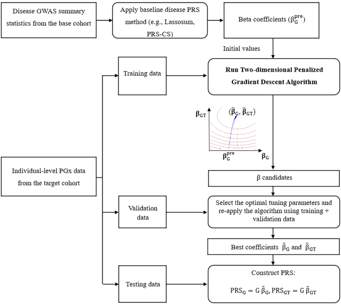
To incorporate the information from the disease GWAS (base) data or jointly analyze the disease GWAS (base) data and the PGx GWAS (target) data, a two-dimensional penalized gradient descent algorithm is further proposed to update \(}\), with initial values \(}}^=[}}_}}^}}\,}}_}}^}}]\) calculated by the model that was pre-trained using disease GWAS:

$$\frac}}}}=-}}^}}\left(}-}}-}\right)+2}},$$

(4)

$$}}^}+1\right)}=}}^}\right)}-}\frac}}}},$$

(5)

$$}}^}+1\right)}=\left(1-2}}\right)}}^}\right)}+2}}}^}}\left(}-}}-}\right),$$

(6)

where \(}\) is the learning rate. For simplicity, we define a new parameter \(}}^}}\,:=2}}\) and choose it from to prevent the term \(\left(1-}}^}}\right)\) from being negative, which would flip the sign of \(}}^}\right)}\) at each iteration and cause instability in the gradient descent updates. We also define \(}}^}}\,:=2}\) to absorb “2”. The new update rule then becomes:

$$}}^}+1\right)}=\left(1-}}^}}\right)}}^}\right)}+}}^}}}}^}}\left(}-}}-}\right).$$

(7)

The learning rate \(}}^}}\) (denote as \(}\) below), regularization parameter \(}}^}}\,\)(denote as \(}\) below), and number of best iteration \(}\) can be tuned and optimized based on the validation dataset (“inner layer”). The learning rate \(}\) controls the step size taken towards minimizing the loss function during optimization. To balance computational cost with effective optimization, we followed Zhao et al.’s suggestion30, selecting \(}\) from a small grid of values: \(\}\}\), where m is the number of variants with non-zero effects in \(}}_}}^}}\). The regularization parameter \(}\in [0,\,1)\) controls the strength of shrinkage applied to the effect sizes. Our chosen values for λ \(\\}\), correspond to no shrinkage, a medium degree of shrinkage, and a large degree of shrinkage, respectively. In addition, the parameter \(n.\), the total number of iterations, is set to 30. Within these 30 iterations, we select the iteration that yields the largest \(^\) as the best. We cap iterations at 30 to prevent overfitting since too many iteration steps would result in overfitting30 and the optimal iteration number (with the largest overall R2 or conditional R2) typically occurs early in the iterative process (Fig. S10).

The PRS-PGx-TL is fit using the two-dimensional penalized gradient descent algorithm. With initial values \(}}_}}^}}\) from the baseline disease PRS methods, we use a gradient descent algorithm to update the prognostic and predictive effects \(}}_}},}}_}}\) simultaneously with the L2 penalty loss function. Of note, L2 regularization was used due to (1) the simplicity to get a closed-form update in the gradient descent algorithm to update all parameters simultaneously, (2) our method is built upon certain baseline disease PRS methods, which allows us to flexibly choose L1-based PRS models as baseline methods. In this case, our method can start from the selected features from baseline models even though itself is L2-based. After applying the four-fold cross-validation to select the optimal parameters, the final weights of PRS-PGx-TL can be outputted. The algorithm was summarized in the following Algorithm 1.

Algorithm 1

Two-dimensional penalized gradient descent algorithm

Preparing pre-trained model: apply baseline disease PRS methods to the disease GWAS summary statistics (base cohort) to get \(}}_}}^}}\).

Input: PRS weights \(}}_}}^}}\), individual-level PGx data \(}=\left[}\,\left(}\times }\right)\right]\) and drug response \(}\). In the presence of non-genetic covariates such as sex, age, and top principal components etc., \(}\) is the residuals of the original drug response by first adjusting covariates and \(}\). Otherwise, \(}\) is the residuals of the original drug response after adjusting \(}\).

Hyperparameters: learning rate \(}\), regularization parameter \(}\), number of iterations parameter \(}\).

Initialization: \(}\) from \(\}}\}\) where m is the number of variants with non-zero effects in \(}}_}}^}}\), \(}\) from \(\\), \(}.}=30\), \(}}^=\left[}}_}}^}}_}}^\right]\) where \(}}_}}^=}}_}}^}}\), \(}}_}}^=}\) or \(}}_}}^}}\).

Main algorithm:

while r < n.iter do

  Update \(}}^}+1)}=(1-})}}^})}+}}}^}}\left(}-}}}^}\right)}\right)\),

    \(}}_}}^})}\) could be fixed at \(}}_}}^\) or updated in each iteration here.

end

Parameter tuning:

Divide the training dataset into 4 folds for cross-validation

  In each fold, train the model using the main algorithm on 3 folds, keep \(}}^,\ldots ,}}^}.})}\) for each \(}\) and \(}\) combination, and validate on the remaining fold:

    Calculate \(}}}_}}=\) \(}}}_}}\), \(}}}_}}=\) \(}}}_}}\),

    Calculate the \(}}^}}\) for the model \(}}}}_}}}}}_}}}}\) or

      the conditional \(}}^}}\) for the model \(}}}}}_}}}}|}}}_}}\),

  Calculate the average performance (R2 or conditional R2) across all four folds to obtain the cross-validation score for each combination of hyperparameters.

Select the best combination of \(},},}\) based on the best cross-validation score.

Final Training:

Combine all data (training and validation sets), re-apply the main algorithm with the best parameters \(},},}\).

Output: \(\hat}}=[}}}_}}\,}}}_}}]\).

Simulation studies

We conducted extensive simulation studies to benchmark the performance of our proposed transfer-learning-based PRS-PGx-TL method. PRS-PGx-TL with six different implementation strategies were compared with disease PRS approaches (i.e., C + T, Lassosum, and PRS-CS).

We first simulated the true effect sizes in the base and target cohorts simultaneously, following the spike-and-slab distribution:

$$\left(\begin}}_}}\\ }}_}}\\ }}_}}\end\right)|}}_}}=\left\}\left(0,\Sigma \right) & ,\,}}_}}=1\\ 0 & ,\,}}_}}=0\end\right.,}}}_}}\sim }\left(}\right),}=\frac}}_}}^}}}\Omega ,$$

(8)

where \(}}_}}\) denotes the effect size of SNP \(}\) in the base cohort of a disease GWAS and \(}}_}}\) and \(}}_}}\) denote the prognostic and predictive effect sizes of SNP \(}\) (i.e., \(}}_}}\) and \(}}_}}\)) in the target cohort of a PGx GWAS, respectively. \(}\) is the proportion of causal variants, \(}}_}}^\) is the heritability of the trait in the base cohort, and \(}\) is the number of causal SNPs. \(\Omega\) is the correlation matrix, which was set as

$$\Omega |}}_}},}}_}}=\left[\begin1 & }}_}} & }}_}}\times }}_}}\\ }}_}} & 1 & }}_}}\\ }}_}}\times }}_}} & }}_}} & 1\end\right],$$

(9)

where \(}}_}}\) is the prognostic effect correlation between disease GWAS in the base cohort and PGx GWAS in the target cohort. \(}}_}}\) is the correlation between prognostic and predictive effects in the target cohort.

After the true effect sizes in both base (\(}}_}}\)) and target (\(}}_}},\,}}_}}\)) cohorts were simulated, we further simulated disease GWAS summary statistics in the base cohort. Standard deviations (\(}}_}}\)) were extracted from the Global Lipids Genetics Consortium (GLGC) (https://csg.sph.umich.edu/willer/public/glgc-lipids2021/) GWAS summary statistics for the LDL-C trait. We assumed effect sizes from the summary statistics followed a normal distribution \(}}}_}}|}}_}}\sim }(}}_}},}}_}}^)\). p values were calculated as \(}}_}}=2\times (1-}(|}}}_}}/}}_}}|))\), where \(}\) denotes the cumulative density function of a standard normal distribution. We then simulated individual-level PGx data in the target cohort. We set \(}}^=}* }\), where \(}\) is a scale factor that quantifies different magnitudes for the prognostic (\(}\)) and predictive (\(}\)) effects. We used the real genotype matrix (\(}\)) from chromosome 19 of the IMPROVE-IT PGx GWAS data, which includes 20,854 SNPs in total. The drug response was generated following the model:

$$}=}}_}}}+}}+\left(}\times }\right)}}^+},}\sim }\left(0,}}^\right),$$

(10)

where the treatment variable was simulated as T ∼ Bernoulli(0.5) and \(}}^\) was determined by the heritability \(}}_}}^\). In Table S1, we provide details of the parameter setup for \((},\,}}_}}^,\,}}_}},\,}}_}},\,}}_}},\,}}_}}^,})\). After \(}}}_}}\) and \(}}}_}}\) were calculated, we further evaluated the performance of different PRS methods following the model:

$$}}^ }\sim }}}_}}+}}}_}}\times },$$

(11)

where \(}}^ }\) is the residual after adjusting T term. We introduced multiple evaluation criteria, including overall prediction accuracy \(^\), partial \(^\) explained by the \(}}}_}}\) term, partial \(^\) explained by the \(\mathrm}}_}\times T\) term conditional on \(}}}_}}\), \(}}}_}}\)-by-treatment interaction p value, and average treatment effects in different PRS quantiles.

Application to IMPROVE-IT PGx GWAS data

We applied disease PRS methods (C + T, Lassosum, PRS-CS) and the PRS-PGx-TL method with different implementation strategies to predict the drug response (LDL-C log-fold change at 1-month) from the IMPROVE-IT PGx GWAS. IMPROVE-IT is a phase 3b, multicenter, double-blind, randomized study to establish the clinical benefit and safety of Vytorin (Ezetimibe/Simvastatin combined therapy: 10 mg + 40 mg) versus Simvastatin monotherapy (40 mg) in high-risk subjects (registry name: ClinicalTrials.gov, registration number: NCT00202878, and the date of registration: September 13, 2005)31. The ethics committee at each participating center approved the protocol and amendments31. The IMPROVE-IT trial was carried out in accordance with the Declaration of Helsinki, current guidelines on Good Clinical Practices and local ethical and legal requirements31. All participants provided voluntary written informed consent before trial entry31. A completed CONSORT checklist of IMPROVE-IT trial is provided in Table S5. The details of the endpoint, genotyping, genotype QC and imputation for this GWAS analyses are introduced elsewhere19. After GWAS QC and SNP imputation, there were 9,407,967 variants and 6502 subjects remaining. The subjects were further filtered down to 5661 subjects for the GWAS analyses by excluding subjects who had a cardiovascular event prior to month 1, since cardiovascular events prior to this time point may affect LDL-C in a manner unrelated to treatment. After matching SNPs with GLGC data (used as disease GWAS summary statistics) and 1000 Genomes (1000 G) data (used as the reference panel), a total of 1,109,919 SNPs were included for analysis of the LDL-C drug response. Several variables were included as covariates in the analysis model, which included age, gender, prior lipid-lowering (PLL) therapy, early glycoprotein IIb/IIIa inhibition in non-ST-segment elevation acute coronary syndrome (EARLY ACS) trial, high-risk ACS diagnosis, baseline LDL-C level, and five top principal components4,19.

For disease PRS methods, we used the LDL-C disease GWAS summary statistics from GLGC to construct the PRS. For PRS-PGx-TL, we leveraged both the GLGC summary statistics and the IMPROVE-IT PGx data in the PRS construction. Specifically, we first applied the disease PRS methods to the GLGC summary statistics and obtained the SNP weights \(}}_}}^}}\). We then utilized \(}}_}}^}}\) as initial values for the two-dimensional penalized gradient descent algorithm. When applying PRS-PGx-TL methods, we used nested cross-validation procedure as described in section “Results”, and the final PRS for all the patients in the IMPROVE-IT PGx data would be obtained. Finally, we assessed the prediction performance using the same criteria as those in the simulations (overall prediction accuracy \(^\), conditional \(^\), \(}}}_}}\)-by-treatment interaction p value, and average treatment effects in different PRS quantiles for patient stratification evaluation).