Four groups of CBA/CaJ mice (Jackson Laboratories #000654, https://www.jax.org/strain/000654) of either sex (25 male, 32 female) were included in this study: young (n = 17), acute noise exposed (n = 13), aged (n = 14), and aged after noise exposure (n = 13). The goal was to generate a sample of mice that encompassed a wide variety of degrees of cochlear synapse loss with varying degrees of OHC damage. Mice were broadly grouped based on the pattern of synapse loss across the cochlea. Not all mice in a particular group were the same age or experienced the same noise exposure. The young mice were tested between 10 and 42 weeks of age. The acute noise exposed mice were exposed to 94 or 98 dB SPL at 8 weeks of age and were tested between 10 and 13 weeks of age. The aged mice were tested between 82 and 103 weeks of age. The aged after noise exposure mice were noise exposed to 101 dB SPL at 16 weeks of age and were tested between 80 and 104 weeks of age. Both the acute noise exposed and aged after noise exposure groups were exposed to octave-band (8 to 16 kHz) noise for 2 h. All physiological and histological measures were performed in the left ear for each mouse. Mouse data were included in the dataset even if a full set of physiological and histological measures were not available (e.g., 35% of experiments did not measure the SAM and RAM EFR modulated at 1 kHz for a carrier frequency of 32 kHz). All mice previously received a headplate surgery for awake assessment of auditory function for a separate study. Mice were excluded from the study if their DPOAE thresholds at 16 kHz were 10 dB greater than prior to the headplate surgery. Since the goal was to collect data from a sample of mice heterogenous with respect to auditory function, there were no other criteria for exclusion of mice from this study other than health reasons as recommended by a veterinarian.

Noise exposures were performed following Kujawa and Liberman [1]. Awake mice were placed in a custom-built wire cage inside a custom-built noise exposure chamber. The cage was subdivided into six compartments with one mouse per compartment. The cage was positioned on a turntable, ensuring that all mice received a uniform noise exposure that was not affected by the development of standing waves in the chamber. The noise exposure chamber was designed as a trapezoidal prism with only the top and bottom surfaces parallel to each other. Noise exposure was controlled using a custom-written program [20]. Noise stimuli were generated digitally by drawing random samples from a uniform distribution and then bandpass filtered using a 1001 tap finite impulse response filter with a passband of 8 to 16 kHz (> 60 dB/octave slope). To ensure uniform spectral distribution of the noise, the gain of the passband was adjusted to equalize the noise. Stimuli were converted to analog (PCI-6251, National Instruments), amplified (D75-A, Crown Audio), and delivered via a 1-inch compression driver (D220 Ti, JBL Professional Loudspeakers) coupled to a horn (HM25-25, JBL Professional Loudspeakers). Prior to each noise exposure, the intensity level of the noise was calibrated to the target level using a 1/4-inch microphone (377C01 coupled to a 426B03 preamplifier and powered by a 480C02 signal conditioner, PCB Piezotronics).

Animals were anesthetized with a ketamine (100 mg/kg) and xylazine (10 mg/kg) cocktail. Body temperature was monitored rectally and maintained using a heating pad regulated by a homeothermic temperature controller (50-7503F, Harvard Apparatus). A custom-built acoustic system consisting of two speakers and an embedded microphone [21] was positioned inside the intratragal notch just above the external acoustic pore (i.e., the opening of the ear canal). Stimuli were generated digitally using a custom data acquisition program [22], converted to analog (PXI-4461, National Instruments), amplified (SA-1, Tucker-Davis Technologies), high-pass filtered at 500 Hz using a custom-built RC circuit, and delivered to the ear via one of the speakers (CDMG15008-03A, Same Sky [formerly CUI Devices]) in the acoustic system. The embedded microphone (FG-23329-P07, Knowles Electret) was calibrated using a 1/8-inch microphone (46-DP1 powered by a 12AK, GRAS Acoustics). In-ear calibration of the speakers was performed immediately prior to each experiment using the embedded microphone. Responses to ABR and EFR stimuli were collected using needle electrodes (F-E2-12, Natus Medical) positioned at the vertex and intratragal notch with a ground near the tail. Responses were amplified (50,000 ×), band-pass filtered from 10 to 10,000 Hz (P511, Grass Instruments), and digitized (PXI-4461, National Instruments) for further analysis. The full set of physiological measurements were collected in a single session.

ABR stimuli consisted of 5 ms tone pips (0.5 ms cosine-squared rise-fall ramp with 4 ms steady-state). A full stimulus train consisting of a single presentation of each of seven frequencies (5.6 to 45.2 kHz in half-octave steps) and 15 levels (10 to 80 dB SPL in 5 dB steps) was constructed with individual stimuli presented at a rate of 81 per second. Since the ordering of frequencies and levels was arranged in the interleaved ramp design described in Buran et al. [21], which leverages auditory nerve fiber tuning to minimize adaptation, the effective stimulus rate was 11.6 per second for each frequency. ABRs were presented in alternating polarity and a total of 512 artifact-free trials were collected (256 for each polarity). Ensemble averages of ABR waveforms were bandpass filtered at 300 to 3000 Hz and the peak for wave 1 was initially assigned using semi-automated peak-picking software [23] and then reviewed visually by an experienced rater. Raters were blinded to the experimental group. ABR thresholds were identified using an automated algorithm [24].

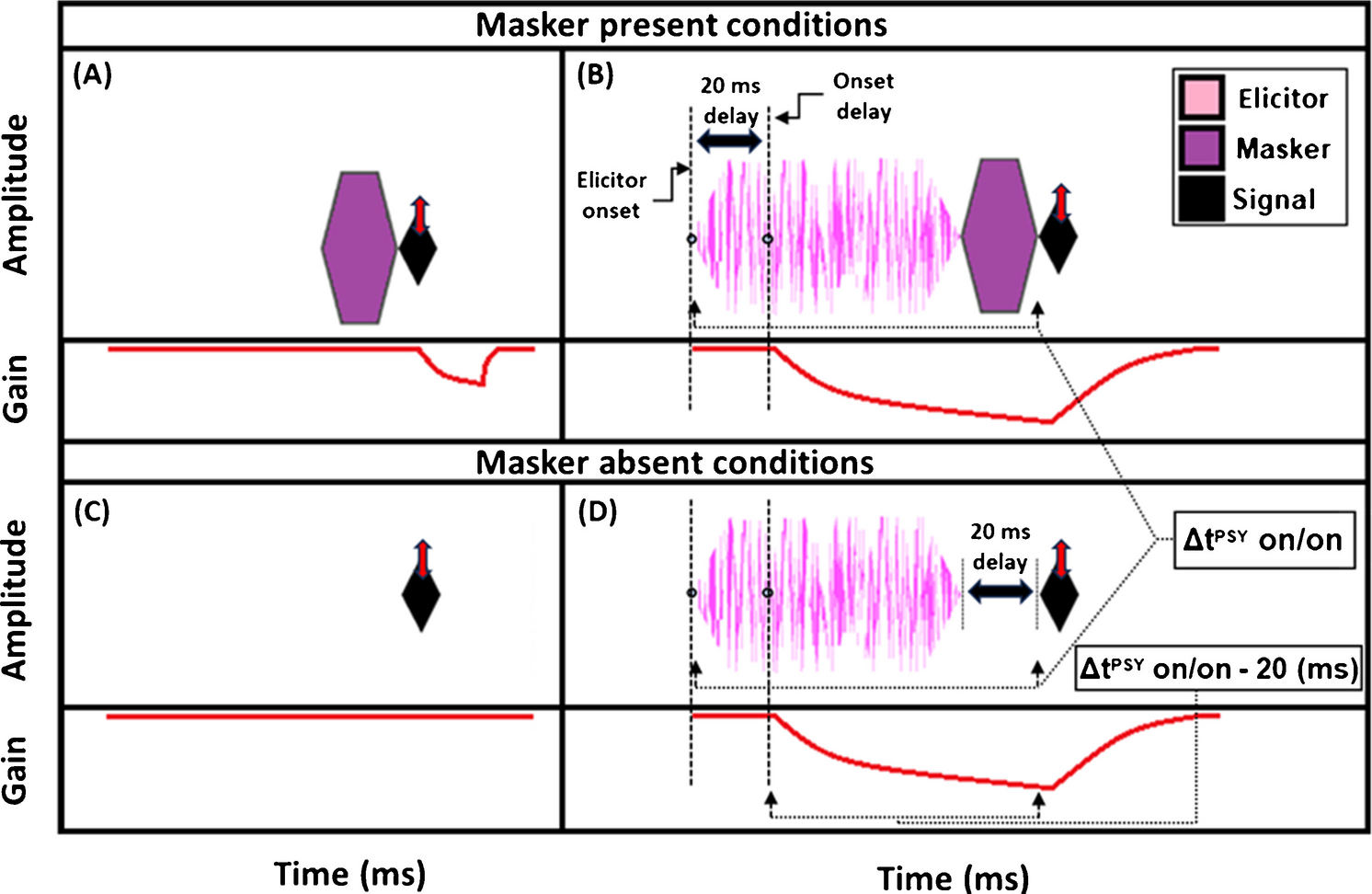
EFR stimuli consisted of 500 ms amplitude-modulated carrier tones with an inter-stimulus interval jittered uniformly between 100 and 120 ms for an average stimulus rate of 1.64/s. Carrier frequencies were 16 or 32 kHz with an overall stimulus level of 70 dB SPL. Stimuli were either sinusoidally (SAM) or rectangular amplitude modulated (RAM) at 110 or 1000 Hz. For SAM tones, the modulation depth was 100%. For RAM tones, stimuli were designed as described in Vasilkov et al. [15] with a modulation depth of 100%, duty cycle of 25%, and a 2.5% Tukey window applied to the onset and offset of each individual cycle of the RAM tone to provide gradual transitions. Stimuli were presented in alternating polarity and a total of 128 trials were collected (64 for each polarity). As illustrated in Fig. 1, different methods of analyzing the EFR data were evaluated due to differences in EFR analysis method across previous studies: (1) compute the magnitude at the modulation frequency (f0); (2) sum the magnitude of the first five multiples of the modulation frequency (f0–4); (3) compute the signal-to-noise ratio (SNR) of the at the modulation frequency relative to the noise floor (f0 dB SNR); (4) sum the magnitude of the first five multiples of the modulation frequency relative to the noise floor (f0–4 dB SNR); and (5) compute the phase locking value (PLV). For f0–4, the values were computed as \(20\cdot\log_\sum\nolimits_^4f_i\) and for f0–4 dB SNR, the values were computed \(20\cdot }__^\frac_}_}\) where \(_\) is the amplitude of the \(i\) th harmonic and \(_\) is the amplitude of the noise floor surrounding the \(i\) th harmonic. Both \(_\) and \(_\) are in units of Vrms. Although it may be considered more correct to sum the powers of the harmonics using the formula \(10\cdot\log_\sum\nolimits_^4f_i^2\), this approach results in a value that is strongly biased towards the frequency components with the largest magnitudes and lowest noise floors, and we found the exact method did not alter our results (Supplemental Data Fig. 1).

Schematic showing EFR stimuli and methods for analyzing the EFR response. Waveforms for SAM (A) and RAM (B) stimuli modulated at 110 Hz. Stimuli are scaled so that the overall RMS for both stimuli is 70 dB SPL. C Magnitude spectrum of the EFR response to a RAM stimulus modulated at 110 Hz illustrating the features that are used in different methods of calculating EFR magnitude, including the noise floor (n0–n4), the modulation frequency (f0) and the first five multiples of the modulation frequency (f0–f4). EFR magnitude can either be extracted at f0 only or by summing f0–4 and can be expressed either as an absolute value (f0, f0–4) or relative to the noise floor (f0 dB SNR, f0–4 dB SNR)

For all methods, EFR magnitude and phase was calculated similarly to the bootstrapping approach described in Zhu et al. [17]. In this approach, 128 trials were drawn with replacement, averaged, and the magnitude spectrum was computed. Random draws were balanced across positive and inverted polarities (i.e., 64 trials from each polarity). This process was repeated 100 times to generate a distribution of the magnitude for each frequency bin. The average value of the distribution at the modulation frequency and the first four harmonics was used to estimate the raw EFR response. To estimate the noise floor, the magnitude in the fourth to seventh discrete Fourier transform (DFT) bin on either side of the frequency of interest was averaged for a total of eight bins.

As an indicator of OHC function, distortion product otoacoustic emissions (DPOAEs) were recorded using the embedded microphone in the acoustic system. For all DPOAE measurements, the f1 level (L1) was fixed at 10 dB higher than the f2 level (L2) and the f2/f1 ratio was fixed at 1.2. DPOAE thresholds were assessed using input–output functions at seven frequencies (5.6 to 45.2 kHz in half-octave steps). For each frequency, the f2 level was swept from 10 to 80 dB SPL in 5 dB steps. Threshold was defined as the f2 level at which the DPOAE level was 0 dB SPL. To parallel the DPOAE measurements often used in human studies of synaptopathy, the DPOAE levels corresponding to L2 values of 40 and 55 dB SPL for f2 = 16 and 32 kHz were also used in the analyses.

Immediately following the physiological measurements, mice were deeply anesthetized, decapitated, and the cochleae extracted for histology. A small hole was made in the apex of the cochleae and 4% paraformaldehyde in phosphate-buffered saline (PBS) at pH 7.3 was perfused through the round window. Cochleae were post-fixed for 2 h at room temperature and then decalcified in 10% ethylenediaminetetraacetic acid (EDTA) for 3–4 days. Once sufficiently decalcified, the cochleae were dissected into five pieces for whole mount immunostaining. Prior to immunostaining, the dissected pieces were cryoprotected in 30% sucrose and then permeabilized using a freeze–thaw step. If immunolabeling could not be initiated immediately, the cochlear pieces were stored at − 80 °C after the initial freezing step. Once thawed, cochlear pieces were rinsed in PBS, blocked with 5% normal horse serum (NHS) in PBS for one hour with 0.3% Triton-X added to further permeabilize the tissue. Primary antibodies were diluted in a solution of 1% NHS in PBS with 0.3% Triton-X. Cochlear pieces were incubated overnight at 37 °C with rabbit anti-MyosinVIIa (dilution of 1:1000, Proteus Biosciences Cat# 25–6790, RRID:AB_10015251), mouse IgG1 anti-CtBP2 (dilution of 1:200, BD Biosciences Cat# 612,044, RRID:AB_399431), and mouse IgG2a Rabbit anti-GluR2 (dilution of 1:2000, Millipore Cat# MAB397, RRID:AB_2113875). Following a wash in PBS, cochleae were incubated for one hour at 37 °C with goat anti-mouse IgG1 AF568 (Thermo Fisher Scientific Cat# A-21124, RRID:AB_2535766), goat anti-mouse Ig2a AF488 (Thermo Fisher Scientific Cat# A-21131, RRID:AB_2535771), and goat anti-rabbit AF647 (Thermo Fisher Scientific Cat# A-21245, RRID:AB_2535813). All secondary antibodies were used at a dilution of 1:1000 in 1% NHS plus 0.3% Triton-X. Following a wash in PBS, the signal was amplified by a second incubation in a freshly-made batch of the same set of secondary antibodies for 1 h at 37 °C. Pieces were washed in PBS and then labeled with 4’,6-diamidino-2-phenylindole (DAPI; Invitrogen D1306) at a dilution of 1:5000. A final wash in PBS was applied prior to mounting and coverslipping the pieces using ProLong Diamond Antifade Mountant (Thermo Fisher P36965).

A cochlear frequency map was computed using a custom program [25] that translates distance along the cochlear partition into frequency using the Greenwood function for mouse [26]. Confocal z-stacks were acquired for each ear at seven frequencies (5.6 to 45.2 kHz in half-octave steps) using a 1.4 NA 63 × oil-immersion objective on either a Zeiss LSM 980 or a Leica TCS SP5 confocal. CtBP2 puncta were identified using Imaris (Oxford Instruments). Assisted by custom software, identified CtBP2 puncta were inspected to identify all CtBP2 puncta paired to a closely apposed glutamate receptor patch (GluR2). Raters were blinded to the experimental group. The percent of CtBP2 puncta identified as orphans (i.e., not paired to a closely apposed GluR2 patch) are shown in Supplemental Data Fig. 2.

All procedures were approved by OHSU’s Institutional Animal Care and Use Committee and conducted in accordance with guidelines from the Office of Laboratory Animal Welfare at the National Institutes of Health. ARRIVE (Animal Research: Reporting of In Vivo Experiments) guidelines were followed in the preparation of this report.

Due to time constraints imposed by the anesthesia, EFR data was only collected for 16 and 32 kHz carriers. Thus, the analysis of the physiological and histological data only include data corresponding to 16 and 32 kHz stimuli or cochlear regions. Data was collected only from the left ear of each mouse to minimize test session duration. Correlations between each of the measures were assessed using the Pearson correlation coefficient from the Python scipy library [27] and confidence intervals computed using the Fisher transformation. The Bonferroni corrected confidence interval was computed as \(\left(1-\frac\right)}\right)\cdot 100\) where \(c\) is the desired confidence interval (95%) and \(n\) is the number of comparisons made [28].

To test the relative ability of each evoked potential measure to predict synapse numbers, we constructed linear regression models based on various combinations of the evoked potential and DPOAE measures, \(_=_+_\cdot }_+_\cdot _+_\).

The number of synapses at the cochlear region corresponding to frequency \(f\) in ear \(i\) is represented by \(_\). The frequency and ear-specific evoked potential measure is represented by \(}_\), the frequency and ear-specific DPOAE measure is represented by \(_\), and the residual error term is represented by \(_\). When testing \(p\) combinations of evoked potential measures (e.g., ABR and EFR), the model was expanded to \(_=_+\sum_^_\cdot } }_+_\cdot _+_\). In this equation, evoked potential measure \(j\) of frequency \(f\) in ear \(i\) is represented by \(} }_\). Models were fit using the Python statsmodels library [29].

Model performance was assessed using ten repeats of ten-fold cross-validation [30]. Cross-validation is a technique used to estimate how well a model will perform on new, unseen data. First, data from the acute noise exposed group of mice were set aside as an independent test set. This was done because these mice have distinct focal synaptopathy and we wanted to specifically evaluate the model’s performance on this condition after training. The remaining data was used for the cross-validation procedure. The data was partitioned into ten folds (i.e., groups). To ensure statistical independence between the training and validation data, all observations from a single ear were assigned to the same fold. For each of the ten iterations, one fold was held out for validation while the model was trained on the pooled data from the other nine folds. The resulting model was then used to predict synapse counts for the held-out validation data. To ensure a more stable and robust estimate of synapse prediction performance, this entire ten-fold process was repeated ten times, with the ears randomly shuffled before partitioning into folds each time. Prediction error was quantified as the root-mean-squared error (RMSE), \(\sqrt_^_-\widehat_}\right)}^}}\), where \(_\) is the \(k\) th synapse count (regardless of frequency), and \(\widehat_}\) is the corresponding prediction. The model was evaluated on both the held-out validation sets and on the separate test set of acute noise exposed mice. The mean and standard error of the RMSE was calculated across all repeats and folds. When presenting results only from the mice with no synaptopathy or broad synaptopathy, RMSE was calculated only for the held-out validation sets. When presenting results only from the mice with focal synaptopathy (i.e., acute noise exposed), RMSE was calculated only for the separate test set of acute noise exposed mice.

The initial models evaluated a total of six different evoked potential options (no evoked potentials, ABR wave 1 amplitude at 80 dB SPL [ABR80], SAM EFR modulated at 110 Hz [SAM110], SAM EFR modulated at 1000 Hz [SAM1000], RAM EFR modulated at 110 Hz [RAM110], and RAM EFR modulated at 1000 Hz [RAM1000]) and four approaches for adjusting for OHC function (no adjustment, DPOAE threshold, DPOAE level at an L2 of 40 dB SPL [DPOAE40], and DPOAE level at an L2 of 55 dB SPL [DPOAE55]).

To establish a baseline for interpreting the prediction error, an intercept-only model (i.e., \(_=_+_\)) was tested in which the predicted synapse number is the average of the observed synapse numbers in the dataset. In addition, because OHC dysfunction is highly correlated with manipulations that reduce synapse numbers (i.e., aging and noise exposure), the ability of DPOAE measures to predict synapse numbers was also evaluated (i.e., \(_=_+_\cdot _+_\)). An ideal metric of synaptopathy would perform better at predicting synapse numbers than the intercept-only and the DPOAE-only models.

Due to known sex differences in ABR wave I amplitude and EFR magnitude in humans [31, 32], we evaluated whether including sex in the models, \(_=_+_\cdot }_+_\cdot _ _\cdot _+_\) where \(}_\) is 1 if the ear is from a female mouse and 0 from a male mouse, would improve synapse predictions. This analysis indicated no improvement in prediction error over models without the sex adjustment (Supplemental Data Fig. 3). For this reason, sex was not included in any further analyses.

Akaike information criterion (AIC) offers complementary information to cross-validation. In contrast to cross-validation, which estimates performance of the model on unseen data, AIC is a model selection tool that offers a relative ranking of models after penalizing for the number of parameters. AIC was calculated on each of these models after fitting to the full dataset. For this approach, the number of observations should be held constant across all models, so all combinations of ear and frequency for which we did not have a full set of observations were dropped, leaving a total of 52 ears (39 when excluding the acute noise exposed group). Since the sample size can be considered small relative to the model degree of freedom, we used a modification of the AIC that corrects for the increased risk of overfitting with small samples (AICc) [33]. For model comparison, the difference in AICc between each model and the best-performing model was calculated (ΔAICc). To interpret the relative strength of evidence for each model, we followed guidelines proposed by Burnham and Anderson [34]. Models with ΔAICc values ≤ 2 are generally considered comparable to the best performing model whereas models with ΔAICc values > 10 indicate a clear preference for the model with a lower AICc. Models with ΔAICc between 2 and 10 should not be rejected outright even though the evidence suggests that the model with a lower AICc is better.