In this section, we review the Coulomb branch geometry relevant to the formulation of topological correlators, the topological twist, and the computation of the contribution from the u-plane to topological correlators.

Notation While we try to keep as much notation from previous literature as possible, we have to introduce various new symbols for the rather detailed universal results of Sect. 3. For functions on the Coulomb branch (or more specifically of the low-energy effective coupling \(\tau \)), we use ordinary Latin letters, such as \(G_(\tau )\). For the values of such functions at the strong coupling singularities, we use the Typewriter font, such as \(\texttt _\). We compiled a list of the most important quantities in Appendix C.

In this subsection, we describe relevant aspects of the Coulomb branch geometries of SQCD with \(N_f\le 3\) massive fundamental hypermultiplets. We do this in a unified way in terms of their Seiberg–Witten solutions.Footnote 6

SW geometry The low-energy effective dynamics of SQCD is famously encoded in the Seiberg–Witten curve, which we list in Appendix B for \(N_f=1,2,3\). The SW curve is fibered over the Coulomb branch (or u-plane) and becomes singular at \(2+N_f\) points, where hypermultiplets become massless. This generalises the solution for pure (\(N_f=0\)) \(\mathcal =2\) super-Yang–Mills theory. In that case, the Coulomb branch has two strong coupling singularities, \(\texttt ^-=-\Lambda _0^2\) and \(\texttt ^+=+\Lambda _0^2\). At \(\texttt ^-\), the monopole becomes massless, while at \(\texttt ^+\) a dyon becomes massless.Footnote 7

The position of the singularities on the u-plane depends in a complicated way on the masses \(}}=(m_1,\dots , m_)\) of the \(N_f\) hypermultiplets. In this article, we consider the case where all masses \(m_i=m\) are equal, and m is large. Since the large mass limit decouples hypermultiplets from the theory, for \(m\rightarrow \infty \) we should then recover the original \(N_f=0\) theory. Thus, when the (equal) mass m of the hypermultiplets is large, this singles out two singularities \(\texttt _^\pm \) which flow to the monopole and dyon singularities \(\texttt _^\pm \rightarrow \pm \Lambda _0^2\) of the pure \(\textrm(2)\) \(\mathcal =2\) theory. The equal mass case is characterised by the Kodaira singular configuration of the Seiberg–Witten curve

$$\begin (I_^,I_1,I_1,I_)~. \end$$

(2.1)

Here, \(I_^\) corresponds to the weak coupling region, and the two \(I_1\)’s become the monopole and dyon singularities for \(m\rightarrow \infty \). The remaining singularities for all \(N_f=1,2,3\) are organised by the flavour symmetry into a single \(I_\) singularity \(\texttt _^*\).

Since in the strict \(m\rightarrow \infty \) limit we obtain the \(N_f=0\) theory, we express the geometry in terms of the scale \(\Lambda _0\) for \(N_f=0\). It is generated in the decoupling limit as a double scaling relation \(m^\Lambda _^=\Lambda _0^4\) [28]. Then for \(N_f=1,2,3\), we have the large m series

$$\begin \begin \texttt _^\pm&=\pm \Lambda _0^2-\frac+\mathcal (m^)~, \\ \texttt _^*&=m^2+\frac+\mathcal (m^)~, \end\end$$

(2.2)

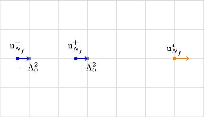
which we depict in Fig. 1.

Large mass singular structure on the Coulomb branch of \(\textrm(2)\) SQCD with \(N_f=1,2,3\) hypermultiplets is as follows. For \(m\gg \Lambda _0\) and positive, the two singularities \(\texttt _^\pm \) approach the two \(N_f=0\) singularities \(\pm \Lambda _0^2\) from below, while the third singularity \(\texttt _^*\) moves to \(+\infty \). In the limit \(m\rightarrow \infty \), this recovers the pure \(N_f=0\) u-plane

The two \(N_f=0\) singularities \(\texttt _^\pm \) are ‘mirrored’ for large m. While \(\texttt _^\pm \) have dimension 2, the quantities \(\texttt _^\pm /m^2\) are dimensionless and admit a Taylor series in \(z\frac\). Let us denote the Taylor series for \(-\texttt _^-/m^2\) by \(T_(z)\). The second singularity is then obtained as

$$\begin -\frac _^+}=T_(-z)~. \end$$

(2.3)

This is because the discriminant \(\Delta _\) of the SW curve depends only on \(z^2\) and is thus invariant under \(z\mapsto -z\), and as a consequence, the two roots \(\texttt _^\pm \) are interchanged. It can be understood as the emergent R-symmetry of the pure \(\textrm(2)\) theory, which acts as a \(\mathbb _2\) symmetry on the u-plane [28, 29].

This article focuses on determining contributions of the vacua \(\texttt _^\pm \) to the topological partition function on four-manifolds. As explained in detail in Sect. 3, due to the symmetry (2.3), it is sufficient to determine the contribution from one singularity only. For the remainder of this section, we focus on the singularity \(\texttt _^-\), where we drop the label in the following and denote it as \(\texttt _\).

Coulomb branch couplings The calculation of topological correlation functions requires various Coulomb branch functions. While some of these functions are obtained directly from the Seiberg–Witten curve, this is not immediately the case for other couplings, such as mass derivatives of the prepotential.

Let us first discuss the more standard Coulomb branch functions: the period \(\frac\) and the physical discriminant \(\Delta _\). These two functions enter the u-plane integral as effective gravitational couplings \(A^\chi B^\sigma \), where A depends only on \(\frac\), while B is given by \(\Delta _^}\). The period \(\frac\) is obtained simply from the SW curve by [50]:

$$\begin \begin \frac=\frac\sqrt\frac}~, \end\end$$

(2.4)

where \(g_2\) and \(g_3\) are the Weierstraß invariants of the Seiberg–Witten curve, as given in Appendix B.1, and \(E_k\) are the Eisenstein series, which we define in (A.4). The physical discriminant [51] is for generic masses defined as the monic polynomial \(\Delta _(u)=\prod _^(u-\texttt _j^*)\), where \(\texttt _j^*\) label the \(2+N_f\) singularities. Using the choice of Weierstraß invariants of Appendix B.1, it is given by

$$\begin \begin \Delta _=(-1)^\Lambda _^(g_2^3-27g_3^2)~, \end\end$$

(2.5)

which up to prefactors is the mathematical discriminant of the SW curve. An important relation between the period \(\frac\) and the discriminant \(\Delta _\) is [52]:

$$\begin \begin \eta ^=2^6(-1)^\Lambda _^\left( \frac\right) ^\Delta _~, \end\end$$

(2.6)

with \(\eta \) the Dedekind eta function (A.6).

The remaining CB functions required for the formulation of topological correlators are most easily expressed as derivatives of the prepotential \(\mathcal \). Since the latter is obtained by a standard calculation, we refer to Appendix B for an exhaustive discussion.

The prepotential of \(\textrm(2)\) QCD with massive hypermultiplets is a function of the masses \(}}\), the coordinate a, and the dynamical scale \(\Lambda _\). While \(\partial ^2 \mathcal /\partial a^2\) gives the effective gauge coupling \(\tau \) of the theory and describes the non-perturbative effective dynamics on flat spacetime, the other second derivatives find an interesting application only in the topological theory.

Let us introduce the couplings \(v_j\) and \(w_\) with \(j,k\in 1,\dots , N_f\) [13,14,15, 53,54,55,56],

$$\begin v_j=\sqrt\frac}~, \qquad w_=2\frac}~. \end$$

(2.7)

They appear in the topological path integral in exponentiated form:

$$\begin D_j=e^~, \qquad C_=e^}~. \end$$

(2.8)

We furthermore require all the second derivatives of the prepotential \(\mathcal \) with respect to \(m_i\) and \(\Lambda _\). These derivatives provide the order parameter u, along with a contact term \(G_\) for the surface observable \(}}\) and the couplings \(H_\) of background fields \(}}_j\) to the surface observable \(}}\) [5, 6, 13, 57],

$$\begin \begin u&=\frac \Lambda _ \frac}}~, \\ G_&=\frac^2}(\Lambda _\partial _})^2 \mathcal ~, \\ H_&=\frac\pi }\frac}\partial m_j}~, \end\end$$

(2.9)

The contact term for the surface observable may be readily evaluated as [5, 6, 57, 58]

$$\begin \begin G_=-\frac^2}E_2\left( \frac\right) ^+\frac^2}\left( u+\frac\delta _\right) ~. \end\end$$

(2.10)

We discuss the calculation of these couplings in depth in Appendix B. Several other important Coulomb branch functions can be extracted either simply from the SW curve, or generally through the prepotential [52].

Couplings at the singularities Naturally, these derivatives and couplings are complicated functions of a, the masses \(}}\) and the scale \(\Lambda _\). For the calculation of partition functions, we are interested in the asymptotic behaviour of the Coulomb branch of SQCD with \(N_f\) equal mass m hypermultiplets, in the regime where m is large. Moreover, under certain circumstances, only their value at the strong coupling singularities is required.

The monopole (dyon) singularity \(\texttt _^\pm \) is approached on the u-plane as \(\tau \rightarrow 0\) (\(\tau \rightarrow 2\)) [52]. Let thus \(\tau _}\) be the local coupling constant, that is, the low-energy effective coupling for the dual photon vector multiplet. For the monopole singularity \(\texttt _^-\), we have \(\tau =-1/\tau _}\), while for the dyon singularity \(\texttt _^+\), we have \(\tau =2-1/\tau _}\). As before, we let \(\texttt _=\texttt _^-\) be the monopole singularity. The vector multiplet scalar for the dual photon then has an expansion

$$\begin \begin u_}(\tau _})=\texttt _+\texttt _ q_}+\mathcal (q_}^2)~, \end\end$$

(2.11)

which is defined as \(u_}(\tau _})=u(-1/\tau _})\), and \(q_}=e^}}\).Footnote 8 The \(q_}\)-series has integer exponents due to the fact that \(\texttt _\) is an \(I_1\) singularity. The first coefficient \(\texttt _\) is of main importance for the calculation later. By expanding the \(\mathcal \)-invariant of the SW curve (B.1) around a singularity \(\texttt _\), the coefficient \(\texttt _\) can be computed as

$$\begin \texttt _=12^3(-1)^\Lambda _^\frac _)^3}'(\texttt _)}~, \end$$

(2.12)

where \(\Delta _'\) is the derivative of \(\Delta _\) with respect to u.

Other important quantities are singular at strong coupling, and we are interested in the finite piece after removing the modular weight factor. The period \(\frac\) has weight 1 and thus is singular at strong coupling. We are interested in the constant term (that is, the coefficient of \(q_}^0\)) in the \(q_}\) series of \((\frac)_}(\tau _})=\tau _}^\frac(-1/\tau _})\). Adding the label \(N_f\) again, it follows from (2.4) thatFootnote 9

$$\begin \texttt _(\tfrac)_}(\tau _})\Big |_}^0}=\frac\sqrt _)} _)}}~. \end$$

(2.13)

Since the prepotential \(\mathcal \) is necessarily fully symmetric in the masses \(}}\), so are the mass derivatives once evaluated at \(m_i=m_j=m\). Therefore, all the single-mass derivatives \(v_j\) (2.7) become identical, and the same holds for the contact terms \(H_\) (2.9). We denote the values of the former couplings at the monopole singularity (up to their weight factor) by \(\texttt _\), while the contact terms become series \(\texttt _\). For the second mass derivatives \(w_\) (or \(C_\)), there are two cases.Footnote 10 This means that in the equal mass limit, there are only two functions: \(C_\) for all j, and \(C_\) for any \(i\ne j\). As we prove below, all those functions become simply a function of \(\Lambda _/m\). More precisely, with \(z=\frac\), we find that they admit Taylor series at \(z=0\) in the variable \(z^}\). In order to distinguish the couplings as global functions (e.g. \(D_j\) and \(C_\)) and their expansions at the monopole singularity for equal masses, we denote the latter by

$$\begin \begin \texttt _&C_^}(\tau _})\big |_}^0}~, \\ \hat }_&C_^}(\tau _})\big |_}^0}~, \\ \texttt _&e^}(\tau _})}\big |_}^0}~, \\ \texttt _&G_^}(\tau _})\big |_}^0}~, \\ \texttt _&H_^}(\tau _})\big |_}^0}~, \\ \texttt _&v_j^}(\tau _})\big |_}^0}~. \end\end$$

(2.14)

for all \(j\ne k=1,\dots , N_f\).Footnote 11 The form of the large mass expansions of those functions is given in (B.21), and as a consequence, the dual functions are holomorphic \(q_}\)-series with integer exponents in a neighbourhood of \(q_D=0\).Footnote 12 Taking the coefficient of \(q_}^0\) is therefore identical to taking the limit \(\tau _}\rightarrow i\infty \). The series \(\texttt _\), \(\hat }_\), \(\texttt _\), \(\texttt _\), \(\texttt _\) together with \(\texttt _\), \(\texttt _\), and \(\texttt _\) form the set of 8 functions required for the contribution of the singularity \(\texttt _\) to the equal mass partition function.

The contact term \(\texttt _\) is straightforward to determine from (2.10),

$$\begin \begin \texttt _&=-\frac^2\texttt _^2}+\frac^2}\left( \texttt _+\frac\delta _\right) ~, \end\end$$

(2.15)

which thus depends only on \(\texttt _\) and \(\texttt _\). The couplings \(\texttt _\), \(\hat }_\) and \(\texttt _\) do not have such a simple expression in terms of the curve, and the determination is one of the key results below.

Before we review the topological twist of \(\mathcal =2\) SQCD, let us set some notation. We are closely following the more recent discussion [14, 15] and refer to [5, 6, 21,22,23, 59, 60] for an overview.

Compact four-manifolds We let X be a smooth, oriented, compact, and simply connected four-manifold. We assume throughout that X has no boundary. Basic topological data of X are its Betti numbers \(b_i=b_i(X)\), Euler number \(\chi \), and signature \(\sigma \). Let L be the embedding of \(H^2(X,\mathbb )\) in \(H^2(X,\mathbb )\otimes \mathbb \), modding out torsion. The intersection form on \(H^2(X,\mathbb )\) provides a bilinear form \(B:L\otimes R\times L\otimes \mathbb \rightarrow \mathbb \) that pairs degree two cocycles, and we abbreviate \(}}_1}}_2B(}}_1,}}_2)\). It furthermore gives rise to a quadratic form \(}}^2B(}},}})\).

For the topological correlators to be nonzero, we require that the moduli space of instantons has even real dimension. Since X is assumed simply connected, this requires that \(b_2^+\) is odd. Moreover, one can deduce that \(H^2(X,\mathbb )\) contains an element c such that \(c^2=2\chi +3\sigma \) [61, p. 377]. The existence of this element implies that X admits an almost complex structure whose first Chern class is c. As a result, X is an almost complex four-manifold, and its tangent bundle is a complex vector bundle [62].

To this holomorphic tangent bundle, we can then associate a Chern character. Let \(T_X^*\) be the cotangent bundle, which is a rank 2 complex vector bundle. The canonical bundle \(K_X=\det (T_X^*)\) has a well-defined first Chern class, which is the canonical class \(K=c_1(K_X)=c_1(T_X^*)=-c_1(T_X)\), and satisfies \(K^2=2\chi +3\sigma \). Finally, we define the holomorphic Euler characteristic \(\chi _}=\frac(\chi +\sigma )\ge 1\), which is an integer for almost complex four-manifolds [2]. To facilitate the comparison with the mathematical literature, we use \((\chi _},K^2)\) rather than \((\chi ,\sigma )\), for which we use the inverse relations \(\chi =-K^2+12\chi _}\) and \(\sigma =K^2-8\chi _}\).

Moreover, we let \(E\rightarrow X\) be a principal \(\text (3)\)-bundle with connection. The second Stiefel–Whitney class \(w_2(E)\in H^2(X,\mathbb _2)\) measures the obstruction to lift E to an \(\textrm(2)\) bundle, which exists globally only if \(w_2(E)=0\). We denote a lift of \(w_2(E)\) to L by \(\bar_2(E)\in L\) and define the ’t Hooft flux \(=\bar_2(E)/2\in L/2\). The instanton number of the principal bundle is defined as \(k=-\frac\int _X p_1(E)\) and satisfies \(k\in -^2 + \mathbb \), where \(p_1\) is the first Pontryagin class.

Topological twist To formulate the massive \(\mathcal =2\) SQCD on a compact four-manifold X, we perform a refined Donaldson–Witten twist. Aside from the usual \(\text (2)\) R-symmetry bundle, for each hypermultiplet we require a principal bundle \(\mathcal _j\) with connection for the flavour symmetries [13, 14, 63].

In the Donaldson–Witten twist, the R-symmetry bundle is isomorphic to the chiral spin bundle \(S^+\). The fields combine to sections of this non-trivial R-symmetry bundle. Effectively, the fields transform under the diagonal group of \(\textrm(2)_+\times \textrm(2)_R\). While the vector multiplet fields combine to differential forms, the hypermultiplet bosons become spinors, that is, sections \(M^j\) of the spin bundle \(S^+\), while the fermions are sections of \(S^+\) and \(S^-\). Thus, the twisted hypermultiplets can a priori only be formulated on four-manifolds which are spin, i.e. \(w_2(X)=0\) [5, 23]. However, if the hypermultiplets are charged under a gauge field, the product of these bundles with \(S^\pm \) may be a \(}^c\) bundle, \(W^+\) or \(W^-\) [9, 13, 23]. The topologically twisted hypermultiplets are then well defined on non-spin four-manifolds X whenever \(\bar_2(X)=\bar_2(E) \mod 2L\) [5]. Thus, generally not all ’t Hooft fluxes \(\) are admissible.

To consider more general ’t Hooft fluxes, we can couple the j’th hypermultiplet to a line bundle \(\mathcal _j\). For this, let \(\mathcal _E^}\) be the line bundle whose sections are components of the fundamental representation of \(\textrm(2)\). For \(\mathcal _j=\mathcal _E\otimes \mathcal _j\), the requirement that \(S^\pm \otimes \mathcal _j^\) is globally well defined is that \(c_1(\mathcal _j)\in \bar_2(X)+\bar_2(E) +2L\) for each j. This is consistent with the above constraints for \(c_1(\mathcal _j)=0\). In the following, we will abbreviate \(}}_j\frac c_1(\mathcal _j)\). Then the topological twist is well defined if [14]

$$\begin }}_j\equiv \frac-\mod L~, \end$$

(2.16)

for each \(j=1,\dots ,N_f\). This can be derived using the general approach of the transfer of structure groups between the twisted and untwisted theories [13, 63]. The combination of the fluxes \(}}_j\) is an example of a “generalised \(}^c\) structure”, introduced in [63].

\(\mathcal \)-fixed equations For our case of interest, the \(\mathcal \)-fixed equations are the non-Abelian monopole equations for gauge group SU(2) with \(N_f\) matter fields in the fundamental representation of the gauge group and coupled to the background line bundles \(\mathcal _j\). They read

(2.17)

where \(T^a\) are the generators of the Lie algebra in the fundamental representation SU(2) [6, 21, 24, 25].

We denote the moduli space of solutions to these equations by \(\mathcal ^,N_f}_(X)\), where we suppress the dependence on the fluxes \(}}_j\), and occasionally drop other dependences. It is known that \(\mathcal \) can become non-compact for vanishing masses [