Hodge Dual Relations

It is useful to recount from the appendix of [15] adjoint differential operators and some Hodge dual relations for forms on \(X\).

The Hodge \(\star \) operator acts on type

$$\begin \star : \Omega ^(X) \rightarrow \Omega ^(X) ~. \end$$

Given k-forms \(\eta \), \(\xi \) and a metric \(}s^2 = g_ }x^m \otimes }x^n\) on \(X\), the Hodge dual defines an inner product

$$\begin (~\cdot ~,~\cdot ~) ~~: ~~ \Omega ^k(X) \times \Omega ^k(X) \rightarrow \mathbb ~, \end$$

with

$$\begin (\eta ,\xi ) \,=\, \frac \int _X \,\text\, \eta ^ \, \xi _ ~. \end$$

(A.1)

Now consider two forms \(\eta _k\) and \(\xi _l\), where the subscript denotes their degree and \(k \le l\),. Contraction is

$$\begin \lrcorner : \Omega ^k(X) \times \Omega ^l(X) \rightarrow \Omega ^(X) ~, \end$$

and acts as follows

$$\begin \eta _k \, \lrcorner \, \xi _l \frac \, \eta ^ \, \xi _} \, }x^} \frac \,\eta ^ \, \xi _ ~. \end$$

An interesting feature of this operator is that it is the adjoint of the wedge product

$$\begin (\sigma _ \, \lrcorner \, \xi _l, \eta _k) \,=\, (\xi _l, \sigma _ \eta _k) ~. \end$$

(A.2)

Recall, the de Rham operator \(}\) can be written

$$\begin }\,=\, }x^m \, \nabla ^}_m ~. \end$$

Using (A.2) and integration by parts

$$\begin ( }\eta , \xi ) \,=\, ( }x^m \, \nabla ^}_m \eta , \xi ) \,=\, ( \nabla ^}_m \eta , \xi ^m ) \,=\, ( \eta , - \nabla ^}_m \xi ^m ) ~. \end$$

It follows that

$$\begin }^\dag \xi _k \,=\,\! - \nabla ^}_m \xi ^m \,=\,\! - \frac \, \nabla ^}_n \xi ^n}_} \, }x^} ~. \end$$

(A.3)

The de Rham differential splits into the sum of Dolbeault operators \(}= + }\). Analogously, the codifferential also splits \(}^\dag = ^\dag + }^\dag \) where

$$\begin \begin&^\dag : \Omega ^(X) \rightarrow \Omega ^(X) \qquad , \qquad ^\dag \,=\,\! - \star }\, \star ~,\\&}^\dag : \Omega ^(X) \rightarrow \Omega ^(X) \qquad , \qquad }^\dag \,=\,\! - \star \, \star ~. \end\end$$

(A.4)

One-forms, type (1, 0):

$$\begin \star \, \eta ^ \,=\,\! -\text \, \eta ^ ~ \frac ~. \end$$

(A.5)

Two-forms, types (2, 0) and (1, 1) :

$$\begin \begin&\star \, \eta ^ \,=\, \eta ^ \, \omega ~,\\&\star \, \eta ^ \,=\,\! -\text \, \eta _}^\mu ~ \frac - \eta ^ \, \omega \,=\, (\omega \, \lrcorner \, \eta ^) ~ \frac - \eta ^ \, \omega ~, \end\end$$

(A.6)

Three-forms, types (3, 0) and (2, 1):

$$\begin \begin&\star \, \eta ^ \,=\,\! - \text \, \eta ^ ~,\\&\star \, \eta ^ \,=\, \text \, \eta ^ - \eta _}^\mu \,^ \, \omega \,=\, \text \, \eta ^ - \text \, (\omega \, \lrcorner \, \eta ^) \, \omega ~, \end\end$$

(A.7)

Four-forms, types (3, 1), and (2, 2)

$$\begin \begin&\star \, \eta ^ \,=\, \! - \text \, \eta _\mu }^ ~,\\&\star \, \eta ^ \,=\, \frac \, \eta _}^ \, \omega + \text \, \eta _}^\mu }^ ~, \end \end$$

(A.8)

The five-form, type (3, 2):

$$\begin \star \eta ^ \,=\, - \frac} \, \eta _}^ ~, \end$$

(A.9)

The six-form (3, 3):

$$\begin \star \eta ^ \,=\, - \frac} ~ \eta _}^ ~. \end$$

(A.10)

From these relations, it follows that the Hodge star squares to

$$\begin \star ^2 \, \eta ^ \,=\, (-1)^ \, \eta ~. \end$$

(A.11)

Connection Symbols on

We enumerate some commonly used connection symbols in heterotic theories. We list the components in complex coordinates. We also give expressions for various divergences which are useful for calculations in the paper.

\(X\) is a complex manifold with complex structure J and hermitian metric g. A vector bundle \(V\rightarrow X\) is hermitian if there is a hermitian inner product on sections of the bundle. For example, \(\mathscr _X\) has a hermitian structure facilitated by the hermitian metric \(}s^2 = 2 g_}} }x^\mu \otimes }x^}\). The bundle is holomorphic (or has a holomorphic structure) if the total space V is a complex manifold with complex structure and the projection map \(\pi : V \rightarrow X\) is holomorphic. That is, fibres consist only of holomorphic sections according to . This is equivalent to the transition functions being purely holomorphic. For example, the bundle \(\mathscr _X\) is not a holomorphic bundle while \(\mathscr _X^\) is a holomorphic bundle.

A connection \(\nabla \) on \(\mathscr _X\) is metric compatible if \(\nabla g = 0\). A connection \(\nabla \) is hermitian if it preserves the hermitian structure. That is, it is metric compatible and \(\nabla J = 0\). In terms of components, a hermitian connection has \(\Gamma _\mu }^\nu }_}= \Gamma _\mu }^}}_\rho = 0\). There may be more than one Hermitian connection.

If V is a holomorphic bundle then a connection \(\nabla \) is compatible with its holomorphic structure if \(\nabla ^ = }\). In terms of components \( \Gamma _}}^\nu }_\rho = 0\). For example, if V is a section of \(\mathscr _X^\), then \(\nabla \) is compatible with the holomorphic structure if \(\nabla ^ V = }x^}\left( _}V^\nu + \Gamma _}}^\nu }_\rho V^\rho \right) _\nu = }V\).

1.1 Levi–Civita

Levi–Civita is the unique metric compatible connection with no torsion (symmetric in lower indices). It is hermitian if the manifold is Kähler but not in general.

$$\begin \begin&\Gamma ^}}_}^}_\rho \frac \, g^}}(_\mu g_}} + _\rho g_}}) g^}} \, _\mu g_}} - \frac H_}^}_ g^}} \, _\rho g_}} + \frac H_}^}_ ~,\\&\Gamma ^}}_}^}}}_ \,=\, 0 ~,\\&\Gamma ^}}_}^}_}} \,=\, \frac \, g^}}(_}} g_}} - _}} g_}}) \,=\, \frac H_}^\nu }_}} ~,\\&\Gamma ^}}_}^}}}_}} \,=\, \frac \, g^}\sigma }(_\mu g_}\sigma } - _ g_}}) \,=\,\! -\frac H_}^}}}_}} ~. \end \end$$

(B.1)

1.1.1 Bismut

The supersymmetry Killing spinor of heterotic supergravity (to first order in \(\,}\)) is covariantly constant with respect to the connection \(\Gamma _m^}= \Gamma _m^} - \fracH_m\). Writing J as a spinor bilinear, it follows that \(\omega \) and J are covariantly constant with respect to this connection \(\nabla ^}J = \nabla ^}\omega = 0\) and so it follows \(\Gamma ^}\) is metric compatible and hermitian. The torsion of \(\Gamma ^}\) is completely antisymmetric and equal to \(H=}^c \omega \), i.e. \(T^m}_ H^m}_\). A geometric statement is that there is a unique connection on \(\mathscr _X\) that is hermitian with completely antisymmetric torsion. This is the Bismut connection.

$$\begin \begin&\Gamma ^}}}_}^}_\rho \,=\, g^}} \, _\rho g_}} \,=\, g^}} \, _\mu g_}} - H_}^}_ ~,\\&\Gamma ^}}}_}^}}}_ \,=\, 0 ~,\\&\Gamma ^}}}_}^}_}} \,=\, 0 ~,\\&\Gamma ^}}}_}^}}}_}} \,=\, g^}\sigma } (_\mu g_}} - _\sigma g_}}) \,=\,\! - H_}^}}}_}} ~. \end\end$$

(B.2)

1.1.2 Hull

While the spinor in heterotic is covariantly constant with respect to \(\Gamma ^}\), a different connection \(\Gamma ^}\) appears in the heterotic action. It is not hermitian but has completely antisymmetric torsion with opposite sign \(-H\). Hence, \(\Gamma _m^}= \Gamma _m^} + \fracH_m\). This we call the Hull connection.

$$\begin \begin&\Gamma ^}}}_}^}_\rho \,=\, g^}} \, _\mu g_}} \,=\, g^}} \, _\rho g_}} + H_}^}_ ~,\\&\Gamma ^}}}_}^}}}_ \,=\, 0 ~,\\&\Gamma ^}}}_}^}_}} \,=\, g^}}(_}} g_}} - _}} g_}}) \,=\, H_\mu }^\nu }_}} ~,\\&\Gamma ^}}}_}^}}}_}} \,=\, 0 ~. \end\end$$

(B.3)

1.1.3 Chern

The Chern connection is the unique connection which is hermitian (\(\nabla g = \nabla J = 0\)) and compatible with the holomorphic structure of \(\mathscr _X^\). The connection has no mixed indices. If the manifold is non-Kähler , then it has torsion.

$$\begin \begin&\Gamma ^}}_}^}_\rho \,=\, g^}} \, _\mu g_}} \,=\, g^}} \, _\rho g_}} + H_}^}_ ~,\\&\Gamma ^}}_}^}}}_ \,=\, 0 ~,\\&\Gamma ^}}_}^}_}} \,=\, 0 ~,\\&\Gamma ^}}_}^}}}_}} \,=\, 0 ~. \end\end$$

(B.4)

1.2 Divergences

The divergence of a vector \(\varepsilon ^\mu \) taken with respect to a generic connection

$$\begin \nabla _\mu \varepsilon ^\mu \,=\, _\mu \varepsilon ^\mu + \varepsilon ^\mu \, \Gamma _\nu }^}_ ~. \end$$

(B.5)

To compute this, we need the following contraction

$$\begin \begin \Gamma ^}}_\nu }^\nu }_\mu&\,=\, _\mu \log } + \frac H_}^ ~,\\ \Gamma ^}}}_\nu }^\nu }_\mu&\,=\, _\mu \log } ~,\\ \Gamma ^}}}_\nu }^\nu }_\mu \,=\, \Gamma ^}}_\nu }^\nu }_\mu&\,=\, _\mu \log } + H_}^\nu ~. \end\end$$

(B.6)

The four choices above give

$$\begin \begin \nabla _\mu ^}\varepsilon ^\mu&\,=\, _\mu \varepsilon ^\mu + \varepsilon ^\mu \, _\mu \log } + \frac \varepsilon ^\mu \, H_}^\nu ~,\\ \nabla _\mu ^}}\varepsilon ^\mu&\,=\, _\mu \varepsilon ^\mu + \varepsilon ^\mu \, _\mu \log } ~,\\ \nabla _\mu ^}}\varepsilon ^\mu \,=\, \nabla _\mu ^}\varepsilon ^\mu&\,=\, _\mu \varepsilon ^\mu + \varepsilon ^\mu \, _\mu \log } + \varepsilon ^\mu \, H_}^\nu \end\end$$

(B.7)

As for the vector-valued form \(\Delta _}}}^\mu \), we have, for a generic connection

$$\begin \nabla _\mu \Delta _}}}^\mu \,=\, _\mu \Delta _}}}^\mu + \Delta _}}}^\mu \, \Gamma _\rho }^\rho }_\mu - \Gamma _\mu }^}}}_}} \, \Delta _}}}^\mu ~, \end$$

(B.8)

and the four choices above give

$$\begin \begin \nabla _\mu ^}\Delta _}}}^\mu& _\mu \Delta _}}}^\mu + \Delta _}}}^\mu \, _\mu \log } + \frac \Delta _}}}^\mu \, H_}^\rho - \frac \Delta ^ \, H_}} ~,\\ \nabla _\mu ^}}\Delta _}}}^\mu&\,=\, _\mu \Delta _}}}^\mu + \Delta _}}}^\mu \, _\mu \log } - \Delta ^ \, H_}} ~,\\ \nabla _\mu ^}}\Delta _}}}^\mu \,=\, \nabla _\mu ^}\Delta _}}}^\mu&\,=\, _\mu \Delta _}}}^\mu + \Delta _}}}^\mu \, _\mu \log } + \Delta _}}}^\mu \, H_}^\rho ~. \end\end$$

(B.9)

1.3 Adjoint of the \(\)-Operator

The \(^\dag \)-operator is defined in (A.4) and acts on a (p, q)–form. We want to derive an expression for it in terms of covariant derivatives analogus to that of \(}^\dag \) in (A.3). It easiest to do this, at least initially, with a hermitian operator as these preserve type. For that reason, we focus on Chern (B.4) and Bismut (B.2).

Given a \((p+1,q)\)-form \(\eta \) and a (p, q)-form \(\xi \), the adjoint is

$$ (\xi \,, \eta ) \,=\, (\xi \,, ^\dag \eta )~, $$

where the inner product is the usual one in (A.1) extended to act on complex forms. Note that

Now,

(B.10)

To integrate by parts, we need to take care of the fact that the divergence theorem involves the Levi–Civita connection: \(\int \nabla _m^\text V^m \,\text= 0\) for any well-defined vector \(V^m\). This involves converting the Chern connection to the Levi–Civita connection

$$ \int \nabla ^\text _\mu V^\mu \,\text\,=\, \int \left\_m V^m \, + H_\rho }^\rho }_\mu V^\mu \right\} \,\text\,=\, \int \left( H_\rho }^\rho }_\mu V^\mu \right) \,\text~. $$

Thence,

$$\begin (\xi \,, \eta )&&\frac \int \xi _}_q} \left\ \nabla _\mu ^\text }}^}_q} H_\rho }^\rho }_\mu }}^}_q} \frac H^}_}}^}_q} \right\} \nonumber \\&\,=\,&(\xi ,^\dag \eta )~; \end$$

(B.11)

so we infer

$$\begin \begin ^\dag \eta ^&\frac \left\ \nabla ^\,\mu } \eta _}_q} H_\rho }^\rho }^\mu \eta _}_q} \frac H_}^\eta _}_q}\right\} }x^}_q}\\&\,=\, - \nabla ^\,\mu } \eta ^_ - H_\rho }^\rho }^\mu \eta ^_ -\frac H^\eta ^_~. \end \end$$

(B.12)

Using (B.2), (B.4), we can rewrite this straightforwardly in terms of Bismut

$$\begin ^\dag \eta ^ \,=\, - \nabla ^}\,\mu } \eta ^_ + H^}\,0,1} \eta _}}^ +\frac H^\eta ^_~. \end$$

(B.13)

We can write this in terms of the Levi–Civita connection however it is more complicated as it is not a hermitian connection. From (A.3), recall \(}^\dag \eta = - \nabla ^\,m} \eta _m\) and that \(}^\dag =^\dag + }^\dag \). As \(\eta \) is a \((p+1,q)\)-form, we can project onto type:

$$ (}^\dag \eta )^ = ^\dag \eta ^ = - \nabla ^\,\mu } \eta _\mu ^ - \nabla ^\,}} \eta _}^ $$

Note the last term is really due to it being non-hermitian. Using (B.1), (B.2), (B.4), we can check this matches the expressions for the Chern and Bismut connections.

Calabi–Yau

In the case of the standard embedding, we have the manifold is Kähler \(}\omega = 0\). In that case, together with it being balanced, we show \(\mathcal _\alpha ^\) vanishes.

The Kähler condition \(}\omega = 0\) has a first-order deformation

$$\begin \begin \,}_\alpha \omega }^&\,=\, 0\\ \,}_\alpha \omega }^ + }\,}_\alpha \omega }^&\,=\, 0\\ }\,}_\alpha \omega }^&\,=\, 0~. \end \end$$

(C.1)

This tells us that

$$\begin \begin }_\alpha \omega ^&\,=\, \psi ^ + \xi _\alpha ^\text \\ }_\alpha \omega ^&\,=\, }\psi ^~, \end \end$$

(C.2)

where \(\xi _\alpha ^\text \) is a harmonic representative of . We use that \(h^ = 0\).

On the other hand, the metric being balanced \(}\omega ^2 = 0\) implies

$$\begin \begin ^\dagger \,}_\alpha \omega }^ - }^\dagger \,}_\alpha \omega }^&\,=\, 0\\ }^\dagger \,}_\alpha \omega }^&\,=\, 0~. \end \end$$

(C.3)

Substituting (C.2) into the first line of (C.3) and taking the inner product with \(\psi ^\) yield

(C.4)

and thus,

$$\begin \begin }_\alpha \omega ^&\,=\, \xi _\alpha ^\text \\ }_\alpha \omega ^&\,=\, 0~. \end \end$$

(C.5)

It follows that \(\overline}_\alpha ^ = -2i }_\alpha \omega }^ = 0\), meaning that on a Calabi–Yau manifold, the only surviving degrees of freedom are

$$\begin \begin&\Delta _\alpha }^\nu ~,\quad }_\alpha \mathcal ~, \quad \mathcal _\alpha ^. \end \end$$

(C.6)

Summary of Universal Geometry

This appendix summarises the universal geometry introduced in [5], fixing the conventions used in the body of this paper. The discussion is local on a smooth patch of the heterotic moduli space \(\mathscr \). In particular, whenever we use coordinates \(y^a\) on \(\mathscr \), or speak about tangent vectors to \(\mathscr \), we mean a local coordinate neighbourhood of a smooth point of the moduli space. No global statement about the existence of a smooth universal family over the whole of \(\mathscr \), nor about finite-dimensional cohomology groups on \(\mathscr \), is assumed here.

To make clear what is assumed and what is determined, we use the following convention throughout this appendix. The local fibration

the Ehresmann connection \(c_a}^m\), the e-basis, the tangibility decomposition, and the animus components of the universal fields are definitions. The restriction to a smooth local patch of \(\mathscr \), the integrability condition \(S=0\) for the almost product structure, the block form of and in the e-basis, and the universal relations

are assumptions of the universal geometry structure used here. The mixed tangibility equations used in the main text, such as the expressions for \(\mathscr _a\), \(}_a A\), \(}_a\Theta \), and the relation between \(c_a}^m\) and \(\Delta _\alpha }^\mu \), are consequences of these definitions and assumptions.

A heterotic vacuum corresponding to a point \(y\in \mathscr \) will be denoted by

$$\begin \textsf_y \,=\, \big ([X_y,\omega _y,\Omega _y],\,[E,A]_y,\,[\mathscr _X,\Theta ]_y,\,H_y\big )~. \end$$

In this notation, which is standard in the recent heterotic literature (e.g. [5, 19] or [4]), E denotes the holomorphic gauge bundle and A the Hermitian–Yang–Mills connection. More precisely, for structure group \(K=E_8\times E_8\), the connection A is a connection on the underlying smooth principal K-bundle, while the condition

defines the holomorphic structure on the associated complexified \(K^}\)-bundle, or on an associated complex representation bundle. We suppress this distinction in the main text and refer simply to the holomorphic bundle E with HYM connection A.

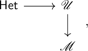
The universal geometry packages a local family of such heterotic vacua over \(\mathscr \) into a fibration \(\mathscr \). We first describe the part of this construction involving the family of complex manifolds. We consider a fibration

(D.1)

whose fibre over \(y\in \mathscr \) is the complex manifold \(X_y\). Topologically, in a sufficiently small neighbourhood in \(\mathscr \), the fibres are diffeomorphic. We choose local coordinates

$$\begin u^M \,=\, (y^a,x^m) \end$$

on , where \(y^a\) are coordinates on \(\mathscr \) and \(x^m\) are coordinates along the fibres.

The vertical tangent bundle is

and is identified fibrewise with \(\mathscr _X\). A choice of horizontal subbundle is equivalent to a choice of Ehresmann connection. We encode this by a projection

(D.2)

In local coordinates,

$$\begin \pi \,=\, \big (}x^m+c_a}^m\,}y^a\big )\otimes _m~. \end$$

Thus,

(D.3)

with adapted frame and coframe

(D.4)

We refer to this as the e-basis. The quantities \(c_a}^m\) are not tensorial under parameter-dependent diffeomorphisms of X; rather, they transform as the components of an Ehresmann connection. If

$$\begin x^m \longrightarrow x^}(x,y)~, \end$$

then

$$\begin c^} \,=\, \frac}}\, c^n - \frac}}\,}y^a~, \end$$

(D.5)

where \(c^m=c_a}^m}y^a\). Consequently

$$\begin e^} \,=\, \frac}}\, e^n~,\qquad e_} \,=\, \frac}}\, e_b~. \end$$

Thus, \(e^m\) and \(e_a\) transform covariantly.

The curvature of the Ehresmann connection is

$$\begin S_}^m \,=\, [e_a,e_b]^m \,=\, c_a}^m}_ - c_b}^m}_ + c_a}^n c_b}^m}_ - c_b}^n c_a}^m}_~. \end$$

(D.6)

The universal geometry used in this paper assumes that the almost product structure determined by \(c_a}^m\) is integrable, namely

$$\begin S_}^m\,=\,0~. \end$$

This assumption does not imply that one may set \(c_a}^m=0\) in the complex coordinates used on . The product structure and complex structure need not be simultaneously diagonal. Indeed, for holomorphic coordinates on the base and fibre one finds

$$\begin \Delta _}}}^\mu \,=\, -_}c_\alpha }^\mu ~, \end$$

(D.7)

so the Ehresmann connection records the variation in the complex structure of the fibres.

Let be an n-form on . In the e-basis, it decomposes as

where p counts the number of \(}y\) legs and q the number of vertical \(e^m\) legs. Explicitly,

(D.8)

The purely vertical component is called the corpus of and is identified with the corresponding form on the fibre \(X_y\). The remaining components, carrying at least one \(}y\) leg, are called the animus components. We refer to [p, q] as the tangibility of the corresponding term.

The de Rham operator on will be denoted

When the product structure is integrable, its decomposition in the e-basis has the schematic form

where \(}\) is the fibrewise exterior derivative and \(}_a\) is the covariant derivative along \(\mathscr \) induced by the horizontal lift \(e_a\). For an ordinary vertical form \(\eta \),

$$\begin }_a\eta \,=\, \mathcal _\eta ~, \end$$

with the result expressed again in the e-basis. After decomposition into complex type, the holotypical derivatives are defined by projection onto complex type:

$$\begin }_\alpha \eta ^ \,=\, \Pi ^\big (\mathcal _\eta \big )~,\qquad }_}\eta ^ \,=\, \Pi ^\big (\mathcal _}}\eta \big )~. \end$$

Thus the notation \(}_\alpha \) is not an ordinary partial derivative on components; it is the horizontal derivative followed by projection to vertical complex type. In coordinates adapted to the e-basis, this is often written as a parameter derivative, but the invariant meaning is the one above.

For bundle-valued quantities, the derivative also uses the animus component of the corresponding universal connection. We write the universal gauge connection as

Similarly,

The curvature of is

and decomposes into tangibility components as

With the conventions above,

$$\begin }_a A \,=\, e_a(A_m)e^m - A_m\,}c_a}^m - }_A A^\sharp _a~, \end$$

where \(}_A=}+[A,\,\cdot \,]\) is the fibrewise gauge-covariant derivative. The pure moduli space curvature component is

In the integrable case, \(S_}^m=0\). The same formulae apply to , with A replaced by \(\Theta \) and by .

Parameter-dependent gauge transformations act on the universal connection in the usual way,

and similarly for with gauge parameter \(\Psi \). Since \(\Phi =\Phi (x,y)\) may depend on the moduli, an ordinary derivative \(_a A\) is not gauge covariant. The role of \(A^\sharp _a\) is precisely to make \(}_a A\) transform covariantly. Small gauge transformations of first-order deformations are equivalently changes of the moduli space connection; with the sign convention used above,

$$\begin A^\sharp _a \longrightarrow A^\sharp _a+\phi _a~,\qquad }_a A \longrightarrow }_a A-}_A\phi _a~. \end$$

The analogous statement holds for \(\Theta ^\sharp _a\). Thus the fixing of small gauge transformations is part of the choice of universal connection. Holomorphic gauge is the choice in which holomorphic deformations of \(\mathcal =A^\) are represented by holomorphic tangent vectors on \(\mathscr \).

The field strength H is related to the two-form B by

$$\begin H \,=\, }B - \frac\,}}\Big (}[A] - }[\Theta ]\Big )~, \end$$

(D.9)

where

$$\begin }[A] \,=\, \text \hspace\!\left( A}A +\frac\, A^3\right) ~. \end$$

Under gauge transformations of A and \(\Theta \), the two-form B transforms so that H is invariant:

$$\begin }^ B \,=\, B + \frac\,}}\Big ( \text \hspace\big (Y A - Z \Theta \big ) + U - W \Big )~, \end$$

(D.10)

where

$$\begin Y\,=\,}\Phi \Phi ^~,\qquad Z\,=\,}\Psi \Psi ^~, \end$$

and

$$\begin }U \,=\, \frac\text \hspace(Y^3)~,\qquad }W \,=\, \frac\text \hspace(Z^3)~. \end$$

Since H is gauge invariant, its parameter variation can be written in the gauge-covariant form

$$\begin _a H \,=\, }\mathscr _a - \frac\,}} \text \hspace\big (}_a A\,F\big ) + \frac\,}} \text \hspace\big (}_a \Theta \,R\big )~. \end$$

(D.11)

The gauge-invariant two-form \(\mathscr _a\) is defined up to the addition of a \(}\)-closed form.

The universal two-form is written in the e-basis as

The universal three-form is defined by

(D.12)

Its mixed component is precisely the gauge-invariant object appearing in first-order deformation theory:

The universal Hermitian form is taken to have no mixed horizontal–vertical component in the e-basis:

The absence of a \(}y^a e^m\) component is a choice of horizontal distribution and is part of the universal geometry ansatz. It should not be confused with the statement that \(c_a}^m\) vanishes. The latter is generally false in the complex coordinates used in this paper, as in (D.7).

1.1 F-Terms and D-Terms in Universal Geometry

As part of the universal geometry ansatz, we assume that satisfies the extended supersymmetry relation and Bianchi identity [5]:

These are part of the defining structure of the universal geometry. Their vertical components reproduce the ordinary heterotic relations on each fibre \(X_y\). Their mixed components encode first- and second-order deformation formulae for the original heterotic compactification, including the relations used in the body of this paper.

It is useful to distinguish two kinds of parameters. The coordinates \(y^a\) label points of the original heterotic moduli space \(\mathscr \). A deformation of the universal geometry itself is a further one-parameter deformation of the total collection of universal fields,

The first-order deformation of the universal geometry has components with different tangibility. Its [1, q] components reproduce first derivatives with respect to the original moduli \(y^a\), while its [2, q] components encode second covariant derivatives with respect to those same moduli. Thus, the “first-order deformation of the universal geometry” is not the same as a first-order deformation in two independent moduli directions; rather, the two moduli indices arise from the tangibility decomposition of fields on .

The D-term conditions are treated differently from the F-term and Bianchi identities above. We impose the HYM and balanced conditions fibrewise on each heterotic vacuum. Thus

$$\begin F^\,=\,0~,\qquad F\omega ^\,=\,0~, \end$$

and the corresponding conditions for \(\Theta \) and for the Hermitian structure hold on \(X_y\). We do not assume, unless explicitly stated, that the total space satisfies a balanced condition in the same sense as the fibres. The D-terms are used to select physical representatives of the fibrewise moduli and to constrain deformations of the universal geometry. In particular, when the main text discusses flatness or vanishing curvature for connections over \(\mathscr \), this refers to the relevant pure moduli space components of the universal curvatures, under the stated gauge choices and fibrewise D-term assumptions. It does not mean that the mixed components

vanish; these mixed components are precisely the first-order deformations of the fibrewise gauge and tangent bundle connections.

Finally, the connection \(\Theta \) is included in the universal geometry because it appears in the Green–Schwarz Bianchi identity. In the physical heterotic moduli problem, however, \(\Theta \) is not an independent modulus: it is taken to be the Hull connection, determined by the underlying geometric fields such as , and . Consequently, deformations of appearing in the universal extension complex should be regarded as auxiliary and non-independent until they are eliminated in favour of the corresponding deformations of the physical heterotic fields.