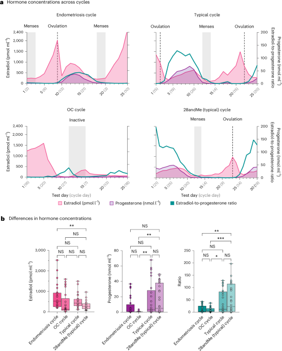
Dense sampling, longitudinal datasets were acquired from three female participants in Jena, Germany. These datasets are referred to as the ‘endometriosis cycle’, ‘typical cycle’ and the ‘OC cycle’. To extend our findings, we also leveraged the open-access 28andMe dataset of one female, which probes the extent to which endogenous fluctuations in sex hormones across a complete reproductive cycle influence the brain33,34,35,36,37,38,40. The data were acquired in Santa Barbara, California, and are referred to as ‘28andMe (typical) cycle’.

For the purposes of control analyses and to probe comparability of our findings, an additional dense sampling, longitudinal dataset of one male was acquired over the time course of 5 weeks in Jena, Germany.

All participants (n = 5) gave written informed consent. The Friedrich Schiller University Jena Ethics Committee (for participants acquired in Jena) and the University of California, Santa Barbara Human Subjects Committee (for participants acquired in Santa Barbara) approved the study. Participants were not compensated. All imaging data are openly available.

ParticipantsPrimary analyses

The study procedures for the participants in Jena, Germany, were as follows: the first healthy female (37 years of age, Caucasian) underwent most weekday testing for five consecutive weeks (9 January–12 February 2023) while freely cycling, resulting in 25 test sessions. The female participant (‘typical cycle’) had a history of regular menstrual cycles (last half-year mean length = 27.1 days, s.d. = 0.64, range = 26–28 days), no history of psychiatric, neurological and endocrine diagnoses, breastfeeding or pregnancy, and no history of alcohol or drug abuse, but the current use of nicotine. The second female participant (30 years of age, Caucasian) diagnosed with endometriosis (‘endometriosis cycle’) participated in this dense sampling, longitudinal study. She received the diagnosis 7 months before the assessments (28 October 2022) after a cyst surgery in the pelvic area. The participant was tracking her menstrual cycle length and reported a mean menstrual cycle length of 24.4 days (s.d. = 1.67, range = 23–27 days) during that time. Otherwise, the female participant had no history of psychiatric or neurological disorders, breastfeeding or pregnancy, and no history of smoking, alcohol or drug abuse. The participant underwent testing from Monday to Friday for five consecutive weeks (12 June–14 July 2023) while freely cycling, resulting in 25 test sessions. The third healthy female (31 years of age, Caucasian) underwent most weekday testing for five consecutive weeks (27 March–28 April 2023), resulting in 25 test sessions. Before the assessments, the participant had been prescribed a combined OC pill (0.03-mg ethinyl-estradiol, 2-mg dienogest, Maxim, Jenapharm) approximately 3 months before study initiation. The female participant (‘OC cycle’) had no history of psychiatric, neurological or endocrine diagnoses, nor had she experienced breastfeeding or pregnancy. Furthermore, she had no history of alcohol or drug abuse and did not use nicotine.

The study procedure for the fourth participant was as follows: a healthy female participant (23 years of age, Caucasian, ‘28andMe (typical) cycle’) underwent testing for 30 consecutive days (9 July–7 August 2018) while freely cycling. She had a history of regular menstrual cycles (no missed periods, cycle occurring every 26–28 days) and had not taken hormone-based medication in the 12 months before the first study. The participant had no history of psychiatric or neurological disorders, breastfeeding or pregnancy, and no history of smoking, alcohol or drug abuse.

Additional analyses (male participant)

The fifth participant, a healthy male (36 years of age, Caucasian), underwent most weekday testing for five consecutive weeks (4 May–7 June 2023), resulting in 25 test sessions. The male participant (‘male’) had no history of psychiatric, neurological or endocrine diagnoses, and reported no instances of alcohol, drug or nicotine abuse.

Image acquisition

For datasets collected in Jena (typical cycle, endometriosis cycle, OC, male), scans were collected at 7.30 a.m. (±30 min) local time. The imaging dataset for the typical cycle was acquired on a 3 T MRI scanner (Prisma, Siemens Medical Solutions; software version MR E11) with a 64-channel head coil. The imaging datasets for the endometriosis cycle, male and female on OC, were acquired on a 3T MRI scanner (Prisma, Siemens Medical Solutions; software version MR XA30) with a 64-channel head coil. Structural MRI for the datasets was acquired with T1w magnetization prepared–rapid gradient echo sequence with the generalized autocalibrating partially parallel acquisitions acceleration. Scan parameters were as follows: echo time = 2.22 ms, repetition time = 2,400 ms, inversion time = 1,000 ms, flip angle = 8°, matrix size = 320 × 320 pixels, field of view = 256 mm, band width = 220 Hz pixel−1 and slice thickness = 0.80 mm.

For the 28andMe (typical) cycle dataset, scans were collected on a 3 T MRI scanner (Prisma, Siemens Medical Solutions; software version MR D13D) equipped with a 64-channel head coil. Structural scans were acquired using a T1w magnetization prepared–rapid gradient echo sequence with the generalized autocalibrating partially parallel acquisitions acceleration with the following parameters: echo time = 2.31 ms, repetition time = 2,500 ms, inversion time = 934 ms, flip angle = 7°, matrix size = 320 × 320 pixels, field of view = 255 mm, band width = 210 Hz pixel−1 and slice thickness = 0.80 mm.

Image preprocessing

The parameters used to acquire the images (for example, sizes, space directions and space origin) and the quality of the images (for example, motion artifacts, ringing, ghosting of the skull or eyeballs, cutoffs, signal drops and other artifacts) were visually inspected. One scan from the endometriosis cycle (test day 8) had to be removed due to artifacts in subcortical structures, corpus callosum and cingulate gyrus (measurements from this test day were excluded for all statistical analyses). The final datasets consisted of 24 T1w images for the endometriosis cycle, 25 T1w images for the typical cycle, 25 T1w images for the OC cycle, 30 T1w images for the 28andMe (typical) cycle and 25 T1w images for the male.

The T1w images were converted from DICOM to NIfTI files using dcm2niix (version v1.0.20170724, https://www.nitrc.org/projects/mricrogl/) and then preprocessed in SPM12 (version r7771, http://www.fil.ion.ucl.ac.uk/spm) and the CAT12 (version 12.9, https://neuro-jena.github.io/cat)55 toolbox using the (plasticity) longitudinal pipeline approach in Matlab (The MathWorks, version R2021b). All T1w images were corrected for bias-field inhomogeneities and initially tissue-classified into gray matter, white matter and cerebrospinal fluid73, followed by an adaptive maximum a posteriori segmentation74, which also accounts for partial volume effects75. The resulting gray and white matter partitions were spatially normalized to MNI space, Geodesic Shooting Registration76. Subsequently, the normalized tissue segments were smoothed using a 6-mm full-width at half-maximum Gaussian Kernel. The extraction of cortical surfaces uses a projection-based thickness method77 to estimate initial cortical thickness and central surface simultaneously. Topological defects are corrected using spherical harmonics78, followed by surface refinement to produce final central, pial and white surface meshes. These surfaces refine the initial thickness measurement using the FreeSurfer metric79. Subsequently, the individual central surfaces are aligned to the FreeSurfer FsAverage template hemisphere, spherically inflated to minimize distortions80 and spherically registered using a two-dimensional DARTEL approach81,82.

Image quality and motion assessment

We conducted a quality assessment of all T1w images using the Image Quality Rating tool (https://neuro-jena.github.io/cat12-help/). Image quality was evaluated based on assigned values, with ratings of 1 and 2 indicating (very) good image quality (grades A and B), while values around 5 and higher suggest problematic image quality (grades E and above). Notably, all assessed images exhibited excellent to good quality (endometriosis cycle—M = 1.407, s.d. = 0.002; typical cycle—M = 1.471, s.d. = 0.002; 28andMe (typical) cycle—M = 1.480, s.d. = 0.002; OC cycle—M = 1.503, s.d. = 0.003; male—M = 1.469, s.d. < 0.001).

Furthermore, mean framewise displacement (FWD), derived from a 12-min resting-state functional scan acquired before the T1w scans, was extracted to indicate motion across the entire scan duration (approximately 55 min). The MRI protocol included a resting-state functional scan for all participants, except for the typical cycle (here the functional scan was replaced with a magnetic resonance spectroscopy scan). Mean FWD was extremely minimal across all participants (endometriosis cycle—M = 0.121 mm, s.d. = 0.009 mm; OC cycle—M = 0.098 mm, s.d. = 0.009 mm; male—M = 0.137 mm, s.d. = 0.011 mm; Supplementary Fig. 1). Mean FWD for the 28andMe (typical) cycle is found elsewhere40 and did not exceed 0.150 mm.

Endocrine procedure

For the datasets acquired in Jena, Germany, a blood draw was immediately followed by the MRI session at 8:30 a.m. (±30 min). One 4.9-ml blood sample was collected in an S-Monovette Serum-GEL (Sarstedt) with a clotting activator/gel at each test session. The sample was clotted at room temperature and centrifuged (2,500g for 10 min) within 2 h. Estradiol (pmol l−1), luteinizing hormone (LH; IU l−1), follicle-stimulating hormone (FSH; IU l−1) and progesterone serum concentrations (nmol l−1) were determined at the Institute of Clinical Chemistry and Laboratory Diagnostics, Jena University Hospital. Estradiol was assessed with the electrochemiluminescence immunoassay (ECLIA) Elecsys Estradiol III Assay. Assay antibodies, measuring ranges (defined by the limit of detection and the maximum of the master curve) and intra-assay precision coefficients of variation for estradiol were as follows: antibodies, two biotinylated monoclonal anti-estradiol antibodies (rabbit), 2.5 ng ml−1 and 4.5 ng ml−1; measuring range, 18.4–11,010 pmol l−1 (5–3,000 pg ml−1); intra-assay precision, ≤8.4% variation coefficient. LH was assessed with the ECLIA Elecsys LH Assay. Assay antibodies, measuring ranges and intra-assay coefficients of variation for LH were as follows: antibodies, biotinylated monoclonal anti-LH antibody (mice), 2.0 mg l−1; measuring range, 0.3–200 mIU ml−1 (0.3–200 IU l−1); intra-assay precision, ≤2.2% variation coefficient. FSH was assessed with the ECLIA Elecsys FSH Assay. Assay antibodies, measuring ranges and intra-assay coefficients of variation for FSH were as follows: antibodies, biotinylated monoclonal anti-FSH antibody (mice), 0.5 mg l−1; measuring range, 0.3–200 mIU ml−1 (0.3–200 IU l−1); intra-assay precision, ≤2.1% variation coefficient. Progesterone was assessed with the ECLIA Elecsys Progesterone III Assay. Assay antibodies, measuring ranges and intra-assay coefficients of variation for progesterone were as follows: antibodies, biotinylated monoclonal antiprogesterone antibody (recombinant sheep), 30 ng ml−1; measuring range, 0.159–191 nmol l−1 (0.05–60 ng ml−1); intra-assay precision, ≤20.7% variation coefficient. All assays were determined on the cobas e 402/801 analyzer (Roche Diagnostics GmbH) and were used according to the manufacturer’s instructions. The reported intra-assay precision and coefficient of variation values are taken from the manufacturer’s package inserts and reflect the analytical performance of the assays. These values are based on Roche’s validation studies and do not represent quality control data generated at the Institute of Clinical Chemistry and Laboratory Diagnostics, Jena University Hospital, Jena, Germany.

For the 28andMe (typical) cycle dataset acquired in Santa Barbara, CA, USA, a licensed phlebotomist inserted a saline-lock intravenous line into the dominant or nondominant hand or forearm. One 10-ml blood sample was collected in a vacutainer SST (BD Diagnostic Systems) each session. The sample was clotted at room temperature for 45 min until centrifugation (2,000g for 10 min) and then aliquoted into three 1-ml microtubes. Serum samples were stored at −20 °C until assayed. Serum concentrations were determined at the Brigham and Women’s Hospital Research Assay Core. Estradiol and progesterone were assessed through LC–MS. Assay sensitivities, dynamic range and intra-assay coefficients of variation (respectively) were as follows: estradiol—1 pg ml−1, 1–500 pg ml−1, <5% relative s.d.; progesterone—0.05 ng ml−1, 0.05–10 ng ml−1, 9.33% relative s.d. FSH and LH levels were determined using chemiluminescent assay (Beckman Coulter). The assay sensitivity, dynamic range and intra-assay coefficient of variation were as follows: FSH—0.2 mIU ml−1, 0.2–200 mIU ml−1, 3.1–4.3%; LH—0.2 mIU ml−1, 0.2–250 mIU ml−1, 4.3–6.4%.

Analysis approach

Please note that measurements from test day 8 of the endometriosis cycle were excluded from all statistical analyses to ensure consistency in the number of test days across all analyses.

Hormone concentrations

Statistical analyses of hormone concentrations were performed using Statistical Package for Social Sciences (SPSS; version 27). First, a one-way multivariate analysis of variance was conducted with estradiol levels, progesterone levels and estradiol-to-progesterone ratio as dependent variables. The fixed factors were the four individuals (endometriosis cycle, OC cycle, typical cycle and 28andMe (typical) cycle). Post hoc analyses of variance and two-tailed t-tests were performed and Bonferroni-corrected.

Structural brain measures

First, SVD was used to extract spatiotemporal patterns from the preprocessed images by decomposing the three-dimensional image sets into spatial patterns (spatial component) and their associated temporal dynamics (time course and temporal component). The spatial patterns represent the brain regions that share similar spatial changes, while the temporal component reflects these changes evolve over time. To ensure consistency in spatial patterns while allowing for distinct temporal patterns, the typical cycle, the 28andMe (typical) cycle, the endometriosis cycle and the OC cycle were modeled together by concatenating the data from these participants. For the male participants, who do not have a menstrual cycle, the SVD was performed separately to account for the unique dynamics.

By using SVD, we can identify and analyze these patterns, revealing coherent time courses across the brain rather than being restricted to an expected change over time. This approach is analogous to applying independent component analysis to resting-state functional MRI data. However, while the motivation here is to identify underlying independent processes or networks, the objective of our study was to decompose the structural data into orthogonal (nonoverlapping) components. Furthermore, SVD provides consistent and repeatable patterns, which are crucial for reproducibility of the results across different datasets.

Using a flexible modeling approach, we assessed the variations in whole-brain volumetric and CSTPs across the monthly period. Specifically, we used a GAM using the ‘mgcv’ package (version 1.9–1) in RStudio (version 2024.04.1 + 748), which allows the independent variable (test days) to influence the outcome through smooth, nonlinear functions, to address potential nonlinear effects in volumetric and cortical thickness brain dynamics. The default value of k = 10 was used to determine the smoothness of the functions. This approach acknowledges the anticipated complexity and nonlinearity of the relationship between the menstrual cycle and brain structure, enabling a more adaptable modeling of menstrual cycle-dependent trajectories in structural brain dynamics. Initially, we also considered models with autoregressive terms to account for potential temporal dependencies in the data. However, model checks indicated that including autoregressive terms led to overfitting. There, we opted for the simpler GAM model, which provided a more reliable and interpretable fit. The following GAMs were fitted for the VSTPs for each individual separately:

The following GAMs were fitted for the CSTPs for each individual separately (CSTP3 in the male only):

GAMs were adjusted for multiple comparisons using the FDR method83.

Next, we assessed the relationship between the dynamics of volumetric and cortical thickness and gonadal hormones. To stabilize variances, gonadal hormone levels were transformed using the square root. We then used time-series regression models with VSTPs and CSTPs as dependent variables and the gonadal hormones as predictors in SPSS (version 27). These models captured the relationship between current structural dynamics and current gonadal hormone concentrations. The following time-series regression models were fitted for the VSTP1 for each individual separately:

$$}1=_+_\times }+\varepsilon$$

$$}1=_+_\times }+\varepsilon$$

$$}1=_+_\times }+\varepsilon$$

The same time-series regression models were fitted for VSTP2 and VSTP3, as well as CSTP1 and CSTP2 for each individual separately (CSTP3 in the male only). Additionally, we explored functional regression analyses incorporating autoregressive terms to account for potential dependencies in the data. However, model checks indicated that including autoregressive terms resulted in overfitting. As a result, we decided to use the initial simpler model without these terms. Finally, because not all variables were normally distributed, relationships were further investigated using nonparametric Spearman rank correlation, as implemented in the ‘stats’ package (version 4.4.0) in RStudio (version 2024.04.1 + 748). Results were highly consistent across both approaches. All models were adjusted for multiple comparisons using the FDR method83.

Finally, to investigate the association between hormonal concentrations and structural brain measures at each voxel or vertex, we performed a statistical analysis using a general linear model in CAT12. Hormonal concentrations were included as the dependent variable in a regression framework. To identify statistically significant effects, we used the threshold-free cluster enhancement method (https://neuro-jena.github.io/software.html#tfce)84, which integrates both the magnitude and spatial extent of effects and controls for multiple comparisons by applying a family-wise error correction with a significance threshold of P < 0.01. For voxel-wise analyses, voxels with an absolute threshold below 0.1 were excluded to focus exclusively on gray matter regions.

Reporting summary

Further information on research design is available in the Nature Portfolio Reporting Summary linked to this article.