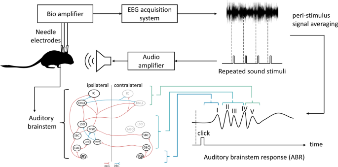
The ABR recording procedures used in this study are similar to the approaches described in previous publications [16,17,18] and illustrated in Fig. 1. ABRs were measured from Fmr1-KO mice (N = 19, 9 females) and C57BL/6 wildtype mice (N = 10, 3 females) with an age range of 70.7 ± 13.3 (Mean ± SD) days old. For gerbil data, 39 young (ages between P60 and P109, 13 females) and 23 old (ages between P750 and P1167, 11 females) gerbils were included. Animals were anesthetized with a mixture of ketamine and xylazine via intraperitoneal injections and placed on a water heating pad maintained at 38 °C (HTP-1500, Heat Therapy Pump, Loudon, TN, USA). Evoked potentials were recorded using platinum subdermal needle electrodes simultaneously placed under the skin at the apex (the top of the skull, midpoint along the interaural axis between the ears; non-inverting), two recording sites behind the two pinna (inverting), nape (reference), and back leg (common). The three active sites were recorded on independent channels, with the apex channel used for the subsequent analyses.

Schematic of the ABR recording setup (top) and sources of ABR waves (bottom)

Sound stimuli were generated as electrical rectangular pulses of 200 µs duration with an interstimulus interval of 35 ± 5 ms (mean ± SD). The stimulus waveform, shaped by the speaker and tubing system, had an effective duration of ~ 0.4 ms (including ringing). Stimuli were delivered using a pair of MF-1 loudspeakers (Tucker Davis Technologies, Alachua, FL, USA), driven by a customized Python script and amplified prior to delivery. The speakers were configured in a closed-field setup, with sound transmitted via a short length of PVC tubing and inserted into the ear canals through customized ear tips. Acoustic waveforms were concurrently recorded using an ER7C probe microphone (Etymotic, Elk Grove Village, IL, USA) connected to the ear tip. The stimulus levels of clicks were calibrated in peak sound pressure level (pSPL) using the ER7C probe microphone and a 94 dB SPL, 1000 Hz tone reference.

Recorded traces were filtered using a 50–3000 Hz second-order bandpass Butterworth filter and averaged across 1000 repetitions per condition, i.e., binaural, left monaural, and right monaural. In addition, the binaural hearing and spatial hearing were also assessed by the binaural interaction component (BIC) of the ABR. The BIC was calculated by taking the difference between the sum of the two (left plus right ear) monaural ABRs, minus the ABR recorded with binaural sound stimulation on a point-by-point basis [17, 19]. The responses were initially recorded for 90 dB SPL stimulus presentations and then gradually decreased in 10 dB SPL steps until the threshold level was reached. The threshold was defined as the average of the minimally detectable waveform and the next dB SPL step where a discernible ABR signal emerged in any of the three recorded channels.

All experimental procedures were reviewed and approved by the institutional animal care and use committees (IACUC) of the University of Colorado Anschutz Medical Campus (permit no.00617) and complied with all National Institutes of Health (NIH) and Office of Laboratory Animal Welfare (OLAW) guidelines for the humane treatment of laboratory animals.

Spiking neurons are the most basic building block to construct the expected auditory brainstem model. Multiple spiking neuron models are available, ranging from the leaky integrate-and-fire model, the Izhikevich model [20], up to much more biophysically realistic (and computationally demanding) Hodgkin-Huxley [21] and multicompartment models. Among these options, the conductance-based leaky integrate-and-fire model stands out as both computationally efficient and widely used, offering a strong balance of simplicity and biological plausibility. The dynamic of the membrane potential \(_\) is described by the following equation:

$$_\frac_}=_\left(_-_\right)+_$$

where \(_\) is the membrane potential, \(_\) is the membrane capacitance, \(_\) is the synaptic current, \(_\) is the leaky conductance, and \(_\) is the leaky reversal potential. The leaky integrate-and-fire neuron emits a spike when its membrane potential reaches the firing threshold \(_\), and the membrane potential resets to \(_\) subsequently.

Synapses can be either simulated by a conductance-based model, where the synaptic current is given by the product of the conductance and the driving force,

$$_\text\text}=_\left(_-_\right)+_(_-_)$$

where \(_\) is the excitatory conductance, \(_\) is the inhibitory conductance, \(_\) is the reversal potential of excitatory synapses, \(_\) is the reversal potential of inhibitory synapses, and  \(\tau_e\) and \(\tau_i\) are corresponding time constants. For each incoming spike, the presynaptic membrane induces an increment of postsynaptic conductance (\(\triangle\,g_e\)  or \(\triangle\,g_i\) , dependent on the synapse type).

The reported simulation results were modeled with a conductance-based leaky integrate and fire model with all parameters used listed in Table 1. The excitatory conductance decay time constant (\(_\)= 0.23 ms) was selected to reflect fast AMPA-mediated synaptic kinetics in auditory brainstem circuits specialized for sub-millisecond temporal processing. Consistent with this, electrophysiological recordings report AMPA decay time constants on the order of 0.2 ~ 0.4 ms in bushy cells [22], MNTB neurons [23], and medial superior olive (MSO) neurons [24]. In this framework, postsynaptic spiking is not driven by isolated synaptic events but emerges primarily from convergent, temporally synchronized inputs; thus, a short τₑ enforces coincidence detection rather than sustained temporal integration. Additionally, a uniform refractory period (\(_\text\text}\) = 5 ms) was implemented across modeled nuclei to maintain numerical stability and to limit parameter dimensionality in the large-scale simulations. Although some early auditory neurons can exhibit shorter refractory periods experimentally, the present study focuses on transient onset-evoked population responses to clicks rather than sustained high-rate firing. The refractory period remains configurable for applications requiring nucleus-specific firing dynamics.

The network architecture (Fig. 2) of the auditory brainstem model reported here is based on our previous spiking network model of the MSO circuit [10] extended to simulate the major components of the auditory afferent pathway and auditory nuclei that facilitate ABRs. Model parameters are user adjustable through a parameter file that is read by the modeling software. We explored some of the parameter space in a previous publication to determine the influence each of these parameters has on the model results [10]. The Brian2 simulator [25] was used for the implementation of this network model. In this simulator, the integration method is handled automatically, first attempting to solve the equations exactly for linear equations and then resorting to numerical algorithms such as the Euler method when necessary. The simulation was performed on the supercomputing cluster at the University of Colorado Boulder (Alpine High Performance Computing Cluster) with a time-step of 10 µs for every calculation.

Network architecture of the auditory brainstem model

In this model, sound waves are encoded into cochlear responses using Zilany’s model [26], implemented in the cochlear package [27], which allows for the encoding of arbitrary sound waves such as pure tones, modulated tones, chirps and natural sounds. A 100-µs click with 100 ms inter-stimulus interval was utilized for simulating click ABRs and a 100-µs click was used for the modeling, rather than the slightly longer effective duration click used here for ABR recordings This is consistent with commonly used durations in human and gerbil ABR studies, although shorter durations (20 ~ 25 µs) are also used in mice to better engage higher-frequency hearing. Nonetheless, the empirical ABR threshold, latency and peak amplitude results we obtained here with the longer click replicated prior ABR studies, suggesting that this difference in duration does not alter the ABR measures analyzed in this study. To simulate auditory nerve activity, we used 60% high spontaneous firing fibers, 20% medium spontaneous firing fibers and 20% low spontaneous firing fibers [28]. According to the neural circuit architecture of auditory brainstem [4], cochlear responses encoded from the auditory stimuli are sent to the brain through the auditory nerve (AN) and are received at the cochlear nuclei (CN). In the CN, the spherical bushy cells (SBCs) innervate medial superior olive (MSO) neurons bilaterally, lateral superior olive (LSO) neurons ipsilaterally, and inferior colliculus (IC) neurons contralaterally. Globular bushy cells (GBCs) innervate the contralateral medial nucleus of the trapezoid body (MNTB) and the ipsilateral lateral nucleus of the trapezoid body (LNTB). The MSO receives bilateral excitation from SBCs, contralateral inhibition via MNTB, and ipsilateral inhibition via LNTB. Meanwhile, the LSO receives ipsilateral excitation from SBC and contralateral inhibition via MNTB. Next, MSO innervates IC ipsilaterally and dorsal nuclei of lateral lemniscus (DNLL) bilaterally, and LSO innervates the ipsilateral DNLL and the contralateral IC. Finally, DNLL inhibits bilateral ICs and contralateral DNLL.

In this model, every neural population contained one thousand spiking neurons that stochastically connected to neurons in corresponding populations with a connection probability (\(_\text\text\text\text\text\text}\)), an axonal transmission delay (\(_\text\text\text\text}\)), and a synaptic delay (\(_\text\text}\)). The detailed parameters of the connectivity were adopted from previous studies [10, 24, 29,30,31,32] and are listed in Table 2. The number of 1000 spiking neurons per nucleus does not reflect anatomical cell counts but was chosen to ensure robust population-level waveform estimation. Absolute ABR amplitude scales with population size, whereas latency relationships remain stable across a broad range of population sizes. Connection probabilities are intended to represent effective synaptic drive in a homogeneous point-neuron framework, rather than literal anatomical fiber convergence. For example, while SBCs are often described as receiving input from a small number of auditory nerve fibers, these fibers can form a dominant endbulb synapse plus additional bouton contacts that contribute to aggregate excitatory drive. Likewise, auditory nerve convergence onto bushy-cell classes spans a broad distribution [32, 33], and prior modeling studies have used effective fan-in values to reproduce timing and downstream activation within simplified neuron formalisms [27, 34]. Accordingly, connectivity values here should be interpreted as functional approximations suitable for population-level ABR synthesis.

In this framework, \(_\text\text\text\text}\) represents axonal propagation delay, whereas \(_\text\text}\) represents an effective synaptic transmission latency capturing presynaptic release and postsynaptic activation delays. This decomposition was applied uniformly across all synaptic connections in the network. Delay values in the network were randomly assigned to each synaptic connection using the mean values listed in Table 2 with a standard deviation of 50 µs. The 50 µs standard deviation introduces physiologically plausible temporal dispersion while preserving phase-locked activity characteristic of auditory brainstem circuits. Each simulation run was initialized with an independent random seed governing probabilistic connectivity, neuronal parameter initialization, and auditory nerve activity synthesis. Consequently, each run represents a newly instantiated network driven by newly generated sensory input, analogous to intersubject variability. Reported ABR traces reflect averages across independent simulations to ensure robustness of waveform morphology. The \(_\text\text\text\text}\) of synaptic connections from the contralateral side were estimated by the fiber myelin thickness and varied in the result section.

The population responses of each modeled nucleus (Fig. 3a), driven by the click sound activity, were calculated separately and presented as the peri-stimulus time histograms shown in Fig. 3b, c. The field potentials for each nucleus were approximated from population activity using a kernel-based mapping applied to population spike trains, following approaches used in prior ABR modeling work [12, 13]. This operation assumes linear superposition, namely, that each unit contributes a stereotyped unit response and the macroscopic waveform reflects the summed contribution across the population [11]. In the present implementation, a Gaussian kernel (σ = 0.05 ms) serves as a computationally simple temporal dispersion function rather than a literal unitary extracellular waveform; this is a deliberate simplification in a point-neuron, single-location-per-nucleus source model. A synaptic-current–based formulation is also compatible with this framework, consistent with the view that transmembrane synaptic currents dominate extracellular field potentials [35], and the kernel choice remains user-configurable for alternative unit-response shapes.

Workflow of modeling ABRs. a The auditory brain stem that was modeled. b Peri-stimulus time histograms induced by encoding click sounds averaged across all neurons for each nucleus (trial-averaged population activity). c Approximated field potentials from histograms. d Exponentially attenuated amplitudes and linearly increased latencies for field potentials propagating over distance. e Final ABRs modeled by propagating and integrating field potentials according to the geometric distribution of the nuclei and electrode location

These field potentials were then assumed to have originated at specific spatial locations based on the geometric arrangement of these nuclei in the brain atlas for the desired species such as gerbil [36], mouse [37], or human [38]. The stereotaxic coordinates used for each modeled nucleus, together with the simulated electrode location, are provided in Supplementary Table S1. With the location of the electrode overlaid, the Euclidean distances between nucleus centers and electrodes were calculated, and the field potentials propagated from the nuclei were estimated with amplitudes exponentially attenuating with distance, as well as the propagation latency linearly increasing with distance, assuming 50 m/s (Fig. 3d). This geometric formulation provides a simplified forward model of volume conduction and does not incorporate distributed dipole orientations or tissue anisotropy; thus, the spatial mapping represents an idealized atlas-based configuration rather than subject-specific anatomical reconstruction.

The single-trial ABR traces were then generated through integrating the field potentials of all simulated nuclei at the recording location, and the raw ABR trace was obtained by taking peri-stimulus signals averaged across all single-trial traces (Fig. 3e). Finally, a detrend filter based on the Savitzky-Golay filter was applied. The baseline trend was estimated using a 50 ms window with polynomial order 2, and the detrended signal was obtained by subtracting the estimated trend from the original trace. For visualization, an additional Savitzky-Golay smoothing filter was applied using a 4 ms window with polynomial order 2.

Both left and right auditory brainstem pathways were explicitly simulated in parallel. All ABR traces were generated from the combined bilateral population activity unless otherwise specified. Thus, the simulated ABR represents the integrated contribution of both hemispheres, consistent with experimental recordings obtained from midline scalp electrodes. For simulated binaural interaction component (BIC) analyses, the network architecture remained identical across conditions; only the auditory input differed. Monaural (left-only and right-only) and binaural click stimuli were simulated separately, and the BIC was computed as the algebraic difference between the summed monaural responses and the binaural response on a point-by-point basis, consistent with experimental convention.

Experimentally recorded ABRs were analyzed with the same workflow. The raw traces were first filtered with a Butterworth bandpass filter (100–3000 Hz, 2nd order), and detrended by a Savitzky-Golay filter. Detrending and smoothing were performed using parameters identical to those described in the “Simulated ABRs” section. Then, ABR waves were detected by searching for local maxima, and labeled sequentially. Manual inspections were performed, and adjustments made when misclassification occurred. The cross-correlation (xCorr) ABR thresholds were automatically computed based on curves fitted with sigmoids of the cross-correlations between adjacent sound levels [39]. The peak amplitude, area, latency and inter-peak intervals were measured as the peak metrics for characterizing ABR waves and BIC DN1. Statistical differences in the peak metrics were tested by using the two-sided Mann-Whitney U test at sound levels higher than 70 dB SPL.

To assess potential sex differences in both the aging gerbil and Fmr1-KO mouse datasets, sex was included as a factor in all statistical analyses using two-way ANOVA or Kruskal–Wallis tests, as appropriate. No significant main effects or interactions involving sex were found for ABR thresholds or wave metrics across multiple click levels, so data from males and females were pooled for all analyses and presentation.

The confocal image dataset consisted of 32 slides of the MNTB from 7 young gerbils and 26 slides from 5 old gerbils [18], where the MNTB neurons were identified based on Nissl fluorescence labeling (Neurotrace 425/435), and the MNTB region was segmented manually in FIJI (ImageJ) software based on trapezoidal shape and location. The number of MNTB cells was automatically counted with a customized script using the scikit-image library. Each 2D section of the z-stack was binarized using the Otsu thresholding algorithm [40]. Next, the binarized images were subtracted by the background obtained by the top-hat transform, and processed with a morphological erosion operation. The number of cells of the image was approximated by counting the number of contours detected in the processed image. The mean cell counts over all z-stacks were computed as the number of MNTB cells of the slide.