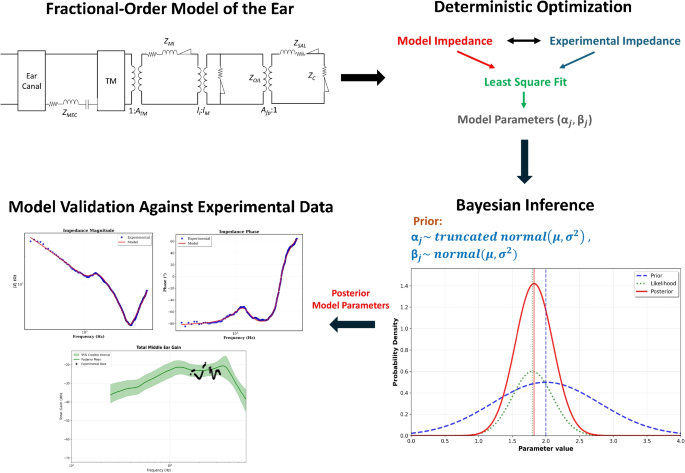
Our Bayesian analysis yielded well-converged posterior distributions for all model parameters. It provided excellent fits to the experimental impedance data and produced credible uncertainty bounds that successfully encompass independent validation measurements.

The construction of appropriate prior distributions is a critical step in Bayesian analysis. Our priors were designed to be informative but not overly restrictive. This approach allows the data to substantially influence the posterior while incorporating reasonable physical constraints and supporting the knowledge gained from the deterministic optimization.

For the fractional-order exponents (\(\alpha _m\), \(\alpha _\), \(\alpha _\), \(\alpha _\)), we assigned truncated normal priors with bounds between 0.5 and 0.999. These bounds ensure that the fractional derivatives remain physically meaningful. The means of these priors were set at the previously optimized values from the deterministic optimization. This reflects our confidence that these values are approximate while acknowledging uncertainty.

The mechanical and electrical parameters including stiffness coefficients (\(K_\), \(K_\), \(K_\), \(K_\)), resistance values (\(R_\), \(R_\), \(R_\), \(R_\)), mass parameters (\(M_\), \(M_\), \(M_\)), and characteristic impedances (\(Z_\), \(Z_\)) were given normal prior distributions. The prior means were set to the deterministic optimization results, and the prior standard deviations were set to 10–20% of the absolute parameter values. We do not expect parameters to vary substantially from their optimized values, but we acknowledge that the optimization may not have found the absolute global minimum or that individual variability exists.

An important practical consideration in MCMC sampling is the numerical stability. Parameters in the model span many orders of magnitude, from very small time constants to large stiffness values. To keep all parameters within computationally stable ranges during the sampling, we applied numerical scaling factors ranging from \(10^\) to \(10^\). For instance, the geometric length parameter \(l_\) was scaled by \(10^3\), and certain time constants were scaled by \(10^6\). These scalings are purely computational conveniences and do not affect the physical interpretation of results—we simply reverse the scaling when reporting final parameter estimates.

The observation noise parameters (\(\sigma _\), \(\sigma _\)) governing the measurement uncertainty in the real and imaginary components of impedance were assigned half-normal priors with scales set to approximately 3% of the respective impedance component standard deviations. This reflects the expected measurement precision of the Mimosa Acoustics reflectance system, which has been characterized in previous studies [48].

Figure 3 shows the posterior distributions for the four fractional-order exponents in the model for subject NDP11. Each panel shows the posterior probability density for one of the fractional-order parameters: (a) \(\alpha _m\) governing the malleus-incus complex, (b) \(\alpha _\) for the stapes-cochlea connection, (c) \(\alpha _\) for the incudostapedial and incudomalleolar joints, and (d) \(\alpha _\) for the tympanic membrane. The vertical dashed line indicates the posterior mean, and the shaded region represents the 95% credible interval.

The posterior distributions exhibit tight, unimodal shapes, indicating that the experimental data are highly informative for these parameters. The unimodal and approximately Gaussian nature of these posterior distributions suggests that simpler approaches, such as using the curvature of the log-likelihood (Fisher information), could provide reasonable estimates of parameter uncertainty in future applications. For this subject, we find \(\alpha _m = 0.840 \pm 0.009\), characterizing the viscoelastic behavior of tissues associated with the malleus. This value indicates substantial viscoelastic effects consistent with the presence of ligaments and muscles attached to this ossicle. The parameter governing the viscoelasticity of the stapes-cochlea connection, \(\alpha _ = 0.980 \pm 0.010\), is very close to one, and given the low standard deviation, this provides strong confidence in a dominant elastic component of the response, consistent with the mechanical behavior of the annular ligament supporting the stapes footplate. The exponent \(\alpha _ = 0.963 \pm 0.015\) characterizes the ossicular joints, ligaments, and muscles, with this near-unity value reflecting dominant elastic behavior arising from the complex joint tissues and surrounding ligaments that permit ossicular mobility while providing support and dissipating energy. Finally, \(\alpha _ = 0.914 \pm 0.020\) describes the tympanic membrane’s viscoelastic characteristics, which is expected given its composite structure of collagen fibers embedded in a viscoelastic matrix. Overall, the narrow credible intervals across parameters indicate strong data informativeness and robust inference.

Figure 4a–o presents the posterior distributions for the remaining model parameters for subject NDP11, including mechanical stiffnesses, resistances, masses, characteristic impedances, and geometric dimensions. Each panel shows the histogram, posterior mean, and 95% credible interval.

All posterior distributions exhibit well-defined, unimodal shapes with reasonable uncertainty bounds. The posterior distributions for the stiffness coefficients show a moderate spread, with coefficients of variation typically in the range of 10–25%. For the NDP11 subject, we observe \(K_ = 4.029 \pm 0.266\), \(K_ = 1.252 \pm 0.163\), and \(K_ = 19.378 \pm 2.762\), which are consistent with the expected variability in biological systems and the uncertainty of measurements. The geometric parameter \(l_ = 18.58 \pm 0.085\) mm shows a very tight posterior distribution with less than 0.5% uncertainty. This makes sense as the length of the ear canal is a relatively stable anatomical dimension that strongly influences the acoustic resonances observed in the impedance measurements. The mass and impedance parameters show posteriors with coefficients of variation ranging from 10 to 25%, similar to the stiffness parameters. The characteristic impedances \(Z_\) and \(Z_\) are particularly important because they influence the impedance transformations at the key interfaces in the system. The symmetric, bell-shaped nature of all these posterior distributions, without significant skewness or multimodality, confirms that the MCMC sampling has adequately converged and thoroughly explored the posterior distribution. This successful parameter estimation provides confidence that the Bayesian framework has appropriately quantified both the central tendency and the uncertainty for all model parameters. Table 1 summarizes the posterior parameter estimates for all seven subjects in the study. Values are scaled, as indicated in the first column, to maintain numerical precision during the computation. This table provides a comprehensive view of inter-subject variability and allows comparison of parameter estimates across individuals.

Several important observations can be made from this cross-subject comparison. There is substantial inter-subject variability in parameter values. This is expected given the natural anatomical and physiological differences between individuals, where stiffness parameters vary by factors of 2–5 across subjects, and fractional-order exponents show ranges from approximately 0.5 to 1.0 depending on the specific parameter and subject. Despite this inter-subject variability in parameter means, the within-subject uncertainties remain relatively consistent, typically 5–25% of the parameter values. This suggests that the Bayesian estimation procedure reliably quantifies uncertainty regardless of the specific parameter values. The length of the ear canal shows remarkably consistent values in most subjects ranging from approximately 18.6 to 22.6 mm, with subject NDP12 as an outlier at 8.9 mm with very tight uncertainty bounds. DP12 was female, and the slightly smaller ear canal size may be associated with individual anatomical differences. Although fractional exponents vary between subjects, there are interesting patterns, where \(\alpha _\) tends to be higher than \(\alpha _\) in most subjects, reflecting differences in their viscoelastic properties. This comprehensive table provides not only a valuable reference for future modeling efforts but also demonstrates the success of the Bayesian approach in handling a diverse population of subjects with varying auditory anatomical and biomechanical properties.

Figures 5, 6, 7, 8, 9, 10, and 11 show the experimental impedance measurements used for the parameter estimation, along with the impedance magnitude and phase predictions by the Bayesian inference using posterior mean parameter values in comparison with the previous deterministic optimization results for all seven subjects. For each subject, the left panel (a) shows the impedance magnitude versus frequency on a log-log plot, while the right panel (b) displays the impedance phase versus frequency on a semi-log plot. The experimental data are overlaid with the Bayesian inference predictions and the deterministic optimization (as seen in the legends).

Posterior distributions for model parameters of NDP11 subject. The parameters include: stiffness coefficients (\(K_\), \(K_\), \(K_\), \(K_\)), the ear canal length (\(l_\)), characteristic impedances (\(Z_\), \(Z_\)), the tympanic membrane time constant (\(T_\)), mass parameters (\(M_\), \(M_\), \(M_\)), and resistance values (\(R_\), \(R_\), \(R_\), \(R_\))

Across all seven subjects, the Bayesian inference accurately captures both the magnitude and phase characteristics of the measured ear impedance across the entire frequency range from approximately 200 Hz to 6 kHz. Table 2 presents a comprehensive comparison of the fitting performance between the Bayesian inference and deterministic optimization across all subjects, quantifying the accuracy using normalized root-mean-square error (NRMSE) for both impedance magnitude and phase.

Impedance fitting for Subject NDP1: (a) impedance magnitude and (b) impedance phase, showing the Bayesian inference (solid red line), deterministic optimization (dashed green line), and experimental data (blue dots) by [40]

Impedance fitting for Subject NDP2: (a) impedance magnitude and (b) impedance phase, showing the Bayesian inference (solid red line), deterministic optimization (dashed green line), and experimental data (blue dots) by [40]

Impedance fitting for Subject NDP3: (a) impedance magnitude and (b) impedance phase, showing the Bayesian inference (solid red line), deterministic optimization (dashed green line), and experimental data (blue dots) by [40]

Impedance fitting for Subject NDP5: (a) impedance magnitude and (b) impedance phase, showing the Bayesian inference (solid red line), deterministic optimization (dashed green line), and experimental data (blue dots) by [40]

Impedance fitting for Subject NDP6: (a) impedance magnitude and (b) impedance phase, showing the Bayesian inference (solid red line), deterministic optimization (dashed green line), and experimental data (blue dots) by [40]

Impedance fitting for Subject NDP11: (a) impedance magnitude and (b) impedance phase, showing the Bayesian inference (solid red line), deterministic optimization (dashed green line), and experimental data (blue dots) by [40]

Impedance fitting for Subject NDP12: (a) impedance magnitude and (b) impedance phase, showing the Bayesian inference (solid red line), deterministic optimization (dashed green line), and experimental data (blue dots) by [40]

The results show substantial improvement of the Bayesian inference over the deterministic optimization. Subjects NDP2, NDP6, and NDP12 show particularly significant improvements in magnitude fitting, where the Bayesian inference reduces errors by factors ranging from 1.9 to 7.3. The magnitude error drops from 19.00% to 2.59%, and the phase error decreases from 16.00% to 7.84% for NDP2. Even in cases where both methods perform well, such as NDP1 and NDP3, the Bayesian inference maintains better accuracy. This consistent improvement across subjects reflects several key advantages of the Bayesian framework: the fractional-order elements more accurately capture the viscoelastic behavior of biological tissues, the HMC sampling procedure efficiently explores the parameter space to identify optimal parameter combinations, and the probabilistic framework naturally incorporates the parameter uncertainty.

In this section, we examine the model’s predictions for the forward and reverse outer-middle ear transfer functions and total gain. In this study, the outer ear only included the ear canal. These quantities characterize how efficiently sound is transmitted through the ear canal and middle ear to reach the cochlea (forward direction) and how effectively cochlear emissions propagate back out to the ear canal (reverse direction).

Figures 12 through 18 present comprehensive transfer function analyses for all seven subjects. Each figure contains three panels showing (a) the forward transfer function magnitude representing sound transmission from the ear canal to the cochlea, (b) the reverse transfer function magnitude showing transmission from the cochlea back to the ear canal, and (c) the stapes velocity transfer function characterizing the velocity of the stapes footplate relative to the ear canal pressure. The shaded regions in each panel represent 95% credible intervals from the Bayesian posterior distribution, illustrating how parameter uncertainty propagates to prediction uncertainty.

Forward (a), reverse (b), and stapes velocity transfer function (c) for NDP1

Forward (a), reverse (b), and stapes velocity transfer function (c) for NDP2

Forward (a), reverse (b), and stapes velocity transfer function (c) for NDP3

Forward (a), reverse (b), and stapes velocity transfer function (c) for NDP5

Forward (a), reverse (b), and stapes velocity transfer function (c) for NDP6

Forward (a), reverse (b), and stapes velocity transfer function (c) for NDP11

Forward (a), reverse (b), and stapes velocity transfer function (c) for NDP12

As can be seen in Figs. 12, 13, 14, 15, 16, 17, and 18, for several subjects and transfer functions, the deterministic optimization estimates fall within the Bayesian 95% credible intervals, indicating agreement between the two approaches and suggesting that the deterministic solutions are consistent with the posterior uncertainty captured by the Bayesian inference. In other cases, the deterministic predictions lie partially or entirely outside the credible intervals, reflecting discrepancies that may arise from point-estimate assumptions in the deterministic optimization and its lack of explicit uncertainty quantification. Overall, these differences highlight the added value of the Bayesian inference in characterizing parameter uncertainty and capturing intersubject variability, particularly in cases where deterministic estimates do not fully align with the probabilistic model predictions.

Model validation against experimental data for all seven subjects: (a) NDP1, (b) NDP2, (c) NDP3, (d) NDP5, (e) NDP6, (f) NDP11, and (g) NDP12. The graphs show the Bayesian inference OMEG estimates (red solid lines), 95% credible intervals (shaded red regions), the estimates by the deterministic optimization (dashed green lines), and the experimental data (black dots) by [40]

Figure 19a–g shows comparisons between the predicted total outer-middle-ear gain (OMEG) of the model and experimental OMEG estimates derived from DPOAE measurements for all seven subjects. In each panel (a–g), the experimental DPOAE-based OMEG estimates are shown by black dots, the predicted OMEG by the Bayesian inference is shown as a solid red line with a shaded 95% credible interval, and the deterministic optimization predictions are shown by dashed green lines.

This validation is important because the OMEG experimental measurements come from a different and independent method than the reflectance measurements, used to estimate the model parameters. The OMEG estimation requires accurate modeling of both forward and reverse sound transmission rather than just the input impedance, and any errors in the model structure or parameter estimates will accumulate through the round-trip path. The results demonstrate excellent agreements across all subjects and frequencies. The model’s 95% credible intervals fully encompass the vast majority of experimental OMEG data points across the entire frequency range. This indicates that the Bayesian uncertainty quantification is well-calibrated with credible intervals that are neither too narrow nor too wide. The agreement between the Bayesian inference and experiment is maintained between approximately 1 and 3.3 kHz, where the OMEG experimental data is available. The predicted OMEG values range between –39 and –17 dB, consistent with experimental observations. This frequency range is also important for hearing, as it includes the region of highest auditory sensitivity. The model accurately captures subject-specific OMEG behavior: for example, NDP1 exhibits a relatively high and stable gain (around –20 dB), whereas NDP11 shows a more frequency-dependent response with a peak near 2 kHz. These differences arise naturally from the subject-specific parameters estimated through Bayesian inference.

The Bayesian inference predictions closely match the deterministic optimization results, and the credible intervals successfully encompass nearly all experimental data points. This excellent agreement across all subjects confirms that the model reliably predicts independent experimental OMEG measurements that were not used during the parameter estimation, demonstrating both a strong predictive capability and well-calibrated uncertainty quantification.

In this section, we compare stapes velocity transfer function and ear canal gain with existing literature.

Figure 20a shows that the present model exhibits a primary resonance near 1 kHz and a secondary elevation around 3–5 kHz. This prediction is consistent with experimental measurements by Voss et al. [49], obtained from 18 normal hearing adult human cadaveric ears, Aibara et al. [50], Nakajima et al. [51], via intracochlear pressure recordings, and Chien et al. [52], based on human and mammalian middle ear transfer function data. Earlier computational predictions by Sun et al. [53] and Gan et al. [54] reproduced the general low-frequency behaviors, but underestimated the secondary resonance, which more recent cavity-inclusive finite-element models by Areias et al. [55] and Garcia Gonzalez et al. [56] captured more clearly. The Bayesian predictions exhibit higher stapes velocity per tympanic membrane pressure above 7 kHz, a frequency region where larger intersubject variability is expected due to anatomical and viscoelastic differences. The variability across parameter sets falls within the experimentally reported intersubject spread, indicating that the Bayesian framework captures realistic biological variations.

Model validation against experimental and computational data. (a) Stapes velocity transfer function [49,50,51,52,53,54,55,56] and (b) ear canal pressure gain [55, 57,58,59] for seven subjects compared with literature as listed in the legend

Figure 20b presents the ear canal pressure gain, which shows a primary resonance between 2.5 and 4 kHz with peak gains of 4–12 dB. These values are lower than the classical results of Wiener et al. [57] (average eardrum pressure ratio in adult males) and Hammershøi and Møller [58] (DPOAE-derived gain, with peaks above 20 dB near 3 kHz), but our predictions align more closely with Mehrgardt and Mellert [59], who measured a resonance near 5 kHz with gains around 14 dB using an impulse-response–based measurement approach. The present model does not reproduce the higher frequency secondary resonance at approximately 8 kHz, observed in the finite-element simulations of Areias et al. [55] or at around 9 kHz, produced in the experimental study by Mehrgardt and Mellert [59]. However, it should be noted that this second resonance was not also observed by Hammershøi and Møller [58]. Moreover, it should be noted that parameter estimation for the current model was performed using impedance data up to 6 kHz. Extending the experimental dataset to a broader frequency range would enable further evaluation and support of the model’s performance at higher frequencies. Comparison with a detailed finite-element model based on the reconstruction of the tympanic membrane, ossicular chain, cochlear load, tendons, ligaments, middle ear joints, portions of the temporal bone, the external auditory meatus, the tympanic cavity, and surrounding soft tissues, the fractional-order model predictions yield lower peak gains but very low intersubject variability [55]. Together, these results demonstrate that the fractional-order Bayesian framework provides stable, physiologically consistent estimates of the ear canal gain while capturing the dominant resonance patterns observed in prior acoustic and computational studies.

MCMC convergence diagnostics for four representative parameters of (a) \(\alpha _\), (b) \(K_\), (c) \(M_\), and (d) \(R_\)

Reliable Bayesian inference requires that the MCMC sampling has ade